This is the multi-page printable view of this section. Click here to print.
Graph
- 1: Best practices for Kusto Query Language (KQL) graph semantics
- 2: Functions
- 2.1: all() (graph function)
- 2.2: any() (graph function)
- 2.3: inner_nodes() (graph function)
- 2.4: labels() (graph function)
- 2.5: map() (graph function)
- 2.6: node_degree_in (graph function)
- 2.7: node_degree_out (graph function)
- 3: Graph exploration basics
- 4: Graph sample datasets and examples
- 5: Graph semantics overview
- 6: Operators
- 6.1: Graph operators
- 6.2: graph-mark-components operator (preview)
- 6.3: graph-match operator
- 6.4: graph-shortest-paths Operator (preview)
- 6.5: graph-to-table operator
- 6.6: make-graph operator
- 7: Scenarios for using Kusto Query Language (KQL) graph semantics
1 - Best practices for Kusto Query Language (KQL) graph semantics
Best practices for graph semantics
Graph semantics supports two primary approaches for working with graphs: transient graphs created in-memory for each query, and persistent graphs defined as graph models and snapshots within the database. This article provides best practices for both methods, enabling you to select the optimal approach and use KQL graph semantics efficiently.
This guidance covers:
- Graph creation and optimization strategies
- Querying techniques and performance considerations
- Schema design for persistent graphs
- Integration with other KQL features
- Common pitfalls to avoid
Graph modeling approaches
There are two approaches for working with graphs: transient and persistent.
Transient graphs
Created dynamically using the make-graph operator. These graphs exist only during query execution and are optimal for ad-hoc or exploratory analysis on small to medium datasets.
Persistent graphs
Defined using graph models and graph snapshots. These graphs are stored in the database, support schema and versioning, and are optimized for repeated, large-scale, or collaborative analysis.
Best practices for transient graphs
Transient graphs, created in-memory using the make-graph operator, are ideal for ad hoc analysis, prototyping, and scenarios where graph structure changes frequently or requires only a subset of available data.
Optimize graph size for performance
The make-graph creates an in-memory representation including both structure and properties. Optimize performance by:
- Apply filters early - Select only relevant nodes, edges, and properties before graph creation
- Use projections - Remove unnecessary columns to minimize memory consumption
- Apply aggregations - Summarize data where appropriate to reduce graph complexity
Example: Reducing graph size through filtering and projection
In this scenario, Bob changed managers from Alice to Eve. To view only the latest organizational state while minimizing graph size:
let allEmployees = datatable(organization: string, name:string, age:long)
[
  "R&D", "Alice", 32,
  "R&D","Bob", 31,
  "R&D","Eve", 27,
  "R&D","Mallory", 29,
  "Marketing", "Alex", 35
];
let allReports = datatable(employee:string, manager:string, modificationDate: datetime)
[
  "Bob", "Alice", datetime(2022-05-23),
  "Bob", "Eve", datetime(2023-01-01),
  "Eve", "Mallory", datetime(2022-05-23),
  "Alice", "Dave", datetime(2022-05-23)
];
let filteredEmployees =
    allEmployees
    | where organization == "R&D"
    | project-away age, organization;
let filteredReports =
    allReports
    | summarize arg_max(modificationDate, *) by employee
    | project-away modificationDate;
filteredReports
| make-graph employee --> manager with filteredEmployees on name
| graph-match (employee)-[hasManager*2..5]-(manager)
  where employee.name == "Bob"
  project employee = employee.name, topManager = manager.name
Output:
| employee | topManager |
|---|---|
| Bob | Mallory |
Maintain current state with materialized views
The previous example showed how to obtain the last known state using summarize and arg_max. This operation can be compute-intensive, so consider using materialized views for improved performance.
Step 1: Create tables with versioning
Create tables with a versioning mechanism for graph time series:
.create table employees (organization: string, name:string, stateOfEmployment:string, properties:dynamic, modificationDate:datetime)

.create table reportsTo (employee:string, manager:string, modificationDate: datetime)
Step 2: Create materialized views
Use the arg_max aggregation function to determine the latest state:
.create materialized-view employees_MV on table employees
{
    employees
    | summarize arg_max(modificationDate, *) by name
}

.create materialized-view reportsTo_MV on table reportsTo
{
    reportsTo
    | summarize arg_max(modificationDate, *) by employee
}
Step 3: Create helper functions
Ensure only the materialized component is used and apply another filters:
.create function currentEmployees () {
    materialized_view('employees_MV')
    | where stateOfEmployment == "employed"
}

.create function reportsTo_lastKnownState () {
    materialized_view('reportsTo_MV')
    | project-away modificationDate
}
This approach provides faster queries, higher concurrency, and lower latency for current state analysis while preserving access to historical data.
let filteredEmployees =
    currentEmployees
    | where organization == "R&D"
    | project-away organization;
reportsTo_lastKnownState
| make-graph employee --> manager with filteredEmployees on name
| graph-match (employee)-[hasManager*2..5]-(manager)
  where employee.name == "Bob"
  project employee = employee.name, reportingPath = hasManager.manager
Implement graph time travel
Analyzing data based on historical graph states provides valuable temporal context. Implement this “time travel” capability by combining time filters with summarize and arg_max:
.create function graph_time_travel (interestingPointInTime:datetime ) {
    let filteredEmployees =
        employees
        | where modificationDate < interestingPointInTime
        | summarize arg_max(modificationDate, *) by name;
    let filteredReports =
        reportsTo
        | where modificationDate < interestingPointInTime
        | summarize arg_max(modificationDate, *) by employee
        | project-away modificationDate;
    filteredReports
    | make-graph employee --> manager with filteredEmployees on name
}
Usage example:
Query Bob’s top manager based on June 2022 graph state:
graph_time_travel(datetime(2022-06-01))
| graph-match (employee)-[hasManager*2..5]-(manager)
  where employee.name == "Bob"
  project employee = employee.name, reportingPath = hasManager.manager
Output:
| employee | topManager |
|---|---|
| Bob | Dave |
Handle multiple node and edge types
When working with complex graphs containing multiple node types, use a canonical property graph model. Define nodes with attributes like nodeId (string), label (string), and properties (dynamic), while edges include source (string), destination (string), label (string), and properties (dynamic) fields.
Example: Factory maintenance analysis
Consider a factory manager investigating equipment issues and responsible personnel. The scenario combines asset graphs of production equipment with maintenance staff hierarchy:
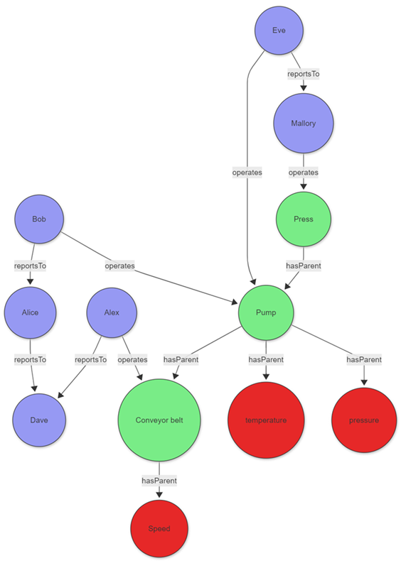
The data for those entities can be stored directly in your cluster or acquired using query federation to a different service. To illustrate the example, the following tabular data is created as part of the query:
let sensors = datatable(sensorId:string, tagName:string, unitOfMeasure:string)
[
  "1", "temperature", "°C",
  "2", "pressure", "Pa",
  "3", "speed", "m/s"
];
let timeseriesData = datatable(sensorId:string, timestamp:string, value:double, anomaly: bool )
[
    "1", datetime(2023-01-23 10:00:00), 32, false,
    "1", datetime(2023-01-24 10:00:00), 400, true,
    "3", datetime(2023-01-24 09:00:00), 9, false
];
let employees = datatable(name:string, age:long)
[
  "Alice", 32,
  "Bob", 31,
  "Eve", 27,
  "Mallory", 29,
  "Alex", 35,
  "Dave", 45
];
let allReports = datatable(employee:string, manager:string)
[
  "Bob", "Alice",
  "Alice", "Dave",
  "Eve", "Mallory",
  "Alex", "Dave"
];
let operates = datatable(employee:string, machine:string, timestamp:datetime)
[
  "Bob", "Pump", datetime(2023-01-23),
  "Eve", "Pump", datetime(2023-01-24),
  "Mallory", "Press", datetime(2023-01-24),
  "Alex", "Conveyor belt", datetime(2023-01-24),
];
let assetHierarchy = datatable(source:string, destination:string)
[
  "1", "Pump",
  "2", "Pump",
  "Pump", "Press",
  "3", "Conveyor belt"
];
The employees, sensors, and other entities and relationships don’t share a canonical data model. The union operator can be used to combine and standardize the data.
The following query joins the sensor data with the time series data to identify sensors with abnormal readings, then uses a projection to create a common model for the graph nodes.
let nodes =
    union
        (
            sensors
            | join kind=leftouter
            (
                timeseriesData
                | summarize hasAnomaly=max(anomaly) by sensorId
            ) on sensorId
            | project nodeId = sensorId, label = "tag", properties = pack_all(true)
        ),
        ( employees | project nodeId = name, label = "employee", properties = pack_all(true));
The edges are transformed in a similar manner.
let edges =
    union
        ( assetHierarchy | extend label = "hasParent" ),
        ( allReports | project source = employee, destination = manager, label = "reportsTo" ),
        ( operates | project source = employee, destination = machine, properties = pack_all(true), label = "operates" );
With the standardized nodes and edges data, you can create a graph using the make-graph operator
let graph = edges
| make-graph source --> destination with nodes on nodeId;
Once the graph is created, define the path pattern and project the required information. The pattern begins at a tag node, followed by a variable-length edge to an asset. That asset is operated by an operator who reports to a top manager via a variable-length edge called reportsTo. The constraints section of the graph-match operator, in this case the where clause, filters the tags to those with an anomaly that were operated on a specific day.
graph
| graph-match (tag)-[hasParent*1..5]->(asset)<-[operates]-(operator)-[reportsTo*1..5]->(topManager)
    where tag.label=="tag" and tobool(tag.properties.hasAnomaly) and
        startofday(todatetime(operates.properties.timestamp)) == datetime(2023-01-24)
        and topManager.label=="employee"
    project
        tagWithAnomaly = tostring(tag.properties.tagName),
        impactedAsset = asset.nodeId,
        operatorName = operator.nodeId,
        responsibleManager = tostring(topManager.nodeId)
Output
| tagWithAnomaly | impactedAsset | operatorName | responsibleManager |
|---|---|---|---|
| temperature | Pump | Eve | Mallory |
The projection in graph-match shows that the temperature sensor exhibited an anomaly on the specified day. The sensor was operated by Eve, who ultimately reports to Mallory. With this information, the factory manager can contact Eve and, if necessary, Mallory to better understand the anomaly.
Best practices for persistent graphs
Persistent graphs, defined using graph models, and graph snapshots, provide robust solutions for advanced graph analytics needs. These graphs excel in scenarios requiring repeated analysis of large, complex, or evolving data relationships, and facilitate collaboration by enabling teams to share standardized graph definitions and consistent analytical results. By persisting graph structures in the database, this approach significantly enhances performance for recurring queries and supports sophisticated versioning capabilities.
Use schema and definition for consistency and performance
A clear schema for your graph model is essential, as it specifies node and edge types along with their properties. This approach ensures data consistency and enables efficient querying. Utilize the Definition section to specify how nodes and edges are constructed from your tabular data through AddNodes and AddEdges steps.
Use static and dynamic labels for flexible modeling
When modeling your graph, you can utilize both static and dynamic labeling approaches for optimal flexibility. Static labels are ideal for well-defined node and edge types that rarely change—define these in the Schema section and reference them in the Labels array of your steps. For cases where node or edge types are determined by data values (for example, when the type is stored in a column), use dynamic labels by specifying a LabelsColumn in your step to assign labels at runtime. This approach is especially useful for graphs with heterogeneous or evolving schemas. Both mechanisms can be effectively combined—you can define a Labels array for static labels and also specify a LabelsColumn to incorporate labels from your data, providing maximum flexibility when modeling complex graphs with both fixed and data-driven categorization.
Example: Using dynamic labels for multiple node and edge types
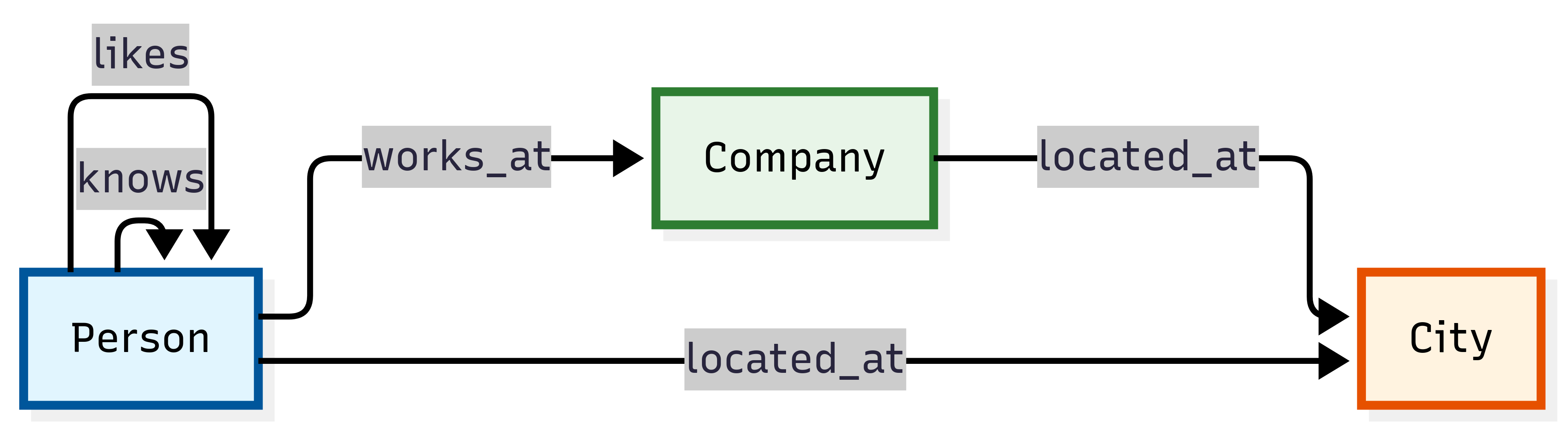
The following example demonstrates an effective implementation of dynamic labels in a graph representing professional relationships. In this scenario, the graph contains people and companies as nodes, with employment relationships forming the edges between them. The flexibility of this model comes from determining node and edge types directly from columns in the source data, allowing the graph structure to adapt organically to the underlying information.
.create-or-alter graph_model ProfessionalNetwork ```
{
  "Schema": {
    "Nodes": {
      "Person": {"Name": "string", "Age": "long"},
      "Company": {"Name": "string", "Industry": "string"}
    },
    "Edges": {
      "WORKS_AT": {"StartDate": "datetime", "Position": "string"}
    }
  },
  "Definition": {
    "Steps": [
      {
        "Kind": "AddNodes",
        "Query": "Employees | project Id, Name, Age, NodeType",
        "NodeIdColumn": "Id",
        "Labels": ["Person"],
        "LabelsColumn": "NodeType"
      },
      {
        "Kind": "AddEdges",
        "Query": "EmploymentRecords | project EmployeeId, CompanyId, StartDate, Position, RelationType",
        "SourceColumn": "EmployeeId",
        "TargetColumn": "CompanyId",
        "Labels": ["WORKS_AT"],
        "LabelsColumn": "RelationType"
      }
    ]
  }
}
```
This dynamic labeling approach provides exceptional flexibility when modeling graphs with numerous node and edge types, eliminating the need to modify your schema each time a new entity type appears in your data. By decoupling the logical model from the physical implementation, your graph can continuously evolve to represent new relationships without requiring structural changes to the underlying schema.
Multitenant partitioning strategies for large-scale ISV scenarios
In large organizations, particularly ISV scenarios, graphs can consist of multiple billions of nodes and edges. This scale presents unique challenges that require strategic partitioning approaches to maintain performance while managing costs and complexity.
Understanding the challenge
Large-scale multitenant environments often exhibit the following characteristics:
- Billions of nodes and edges - Enterprise-scale graphs that exceed traditional graph database capabilities
- Tenant size distribution - Typically follows a power law where 99.9% of tenants have small to medium graphs, while 0.1% have massive graphs
- Performance requirements - Need for both real-time analysis (current data) and historical analysis capabilities
- Cost considerations - Balance between infrastructure costs and analytical capabilities
Partitioning by natural boundaries
The most effective approach for managing large-scale graphs is partitioning by natural boundaries, typically tenant identifiers, or organizational units:
Key partitioning strategies:
- Tenant-based partitioning - Separate graphs by customer, organization, or business unit
- Geographic partitioning - Divide by region, country, or datacenter location
- Temporal partitioning - Separate by time periods for historical analysis
- Functional partitioning - Split by business domain or application area
Example: Multitenant organizational structure
// Partition employees and reports by tenant
let tenantEmployees =
    allEmployees
    | where tenantId == "tenant_123"
    | project-away tenantId;

let tenantReports =
    allReports
    | where tenantId == "tenant_123"
    | summarize arg_max(modificationDate, *) by employee
    | project-away modificationDate, tenantId;

tenantReports
| make-graph employee --> manager with tenantEmployees on name
| graph-match (employee)-[hasManager*1..5]-(manager)
  where employee.name == "Bob"
  project employee = employee.name, reportingChain = hasManager.manager
Hybrid approach: Transient vs. persistent graphs by tenant size
The most cost-effective strategy combines both transient and persistent graphs based on tenant characteristics:
Small to medium tenants (99.9% of tenants)
Use transient graphs for most tenants:
Advantages:
- Always up-to-date data - No snapshot maintenance required
- Lower operational overhead - No graph model or snapshot management
- Cost-effective - No extra storage costs for graph structures
- Immediate availability - No preprocessing delays
Implementation pattern:
.create function getTenantGraph(tenantId: string) {
    let tenantEmployees =
        employees
        | where tenant == tenantId and stateOfEmployment == "employed"
        | project-away tenant, stateOfEmployment;
    let tenantReports =
        reportsTo
        | where tenant == tenantId
        | summarize arg_max(modificationDate, *) by employee
        | project-away modificationDate, tenant;
    tenantReports
    | make-graph employee --> manager with tenantEmployees on name
}

// Usage for small tenant
getTenantGraph("small_tenant_456")
| graph-match (employee)-[reports*1..3]-(manager)
  where employee.name == "Alice"
  project employee = employee.name, managerChain = reports.manager
Large tenants (0.1% of tenants)
Use persistent graphs for the largest tenants:
Advantages:
- Scalability - Handle graphs exceeding memory limitations
- Performance optimization - Eliminate construction latency for complex queries
- Advanced analytics - Support sophisticated graph algorithms and analysis
- Historical analysis - Multiple snapshots for temporal comparison
Implementation pattern:
// Create graph model for large tenant (example: Contoso)
.create-or-alter graph_model ContosoOrgChart ```
{
    "Schema": {
        "Nodes": {
            "Employee": {
                "Name": "string",
                "Department": "string",
                "Level": "int",
                "JoinDate": "datetime"
            }
        },
        "Edges": {
            "ReportsTo": {
                "Since": "datetime",
                "Relationship": "string"
            }
        }
    },
    "Definition": {
        "Steps": [
            {
                "Kind": "AddNodes",
                "Query": "employees | where tenant == 'Contoso' and stateOfEmployment == 'employed' | project Name, Department, Level, JoinDate",
                "NodeIdColumn": "Name",
                "Labels": ["Employee"]
            },
            {
                "Kind": "AddEdges",
                "Query": "reportsTo | where tenant == 'Contoso' | summarize arg_max(modificationDate, *) by employee | project employee, manager, modificationDate as Since | extend Relationship = 'DirectReport'",
                "SourceColumn": "employee",
                "TargetColumn": "manager",
                "Labels": ["ReportsTo"]
            }
        ]
    }
}
```

// Create snapshot for Contoso
.create graph snapshot ContosoSnapshot from ContosoOrgChart

// Query Contoso's organizational graph
graph("ContosoOrgChart")
| graph-match (employee)-[reports*1..10]-(executive)
  where employee.Department == "Engineering"
  project employee = employee.Name, executive = executive.Name, pathLength = array_length(reports)
Best practices for ISV scenarios
- Start with transient graphs - Begin all new tenants with transient graphs for simplicity
- Monitor growth patterns - Implement automatic detection of tenants requiring persistent graphs
- Batch snapshot creation - Schedule snapshot updates during low-usage periods
- Tenant isolation - Ensure graph models and snapshots are properly isolated between tenants
- Resource management - Use workload groups to prevent large tenant queries from affecting smaller tenants
- Cost optimization - Regularly review and optimize the persistent/transient threshold based on actual usage patterns
This hybrid approach enables organizations to provide always-current data analysis for most tenants while delivering enterprise-scale analytics capabilities for the largest tenants, optimizing both cost and performance across the entire customer base.
Related content
2 - Functions
2.1 - all() (graph function)
The all() graph function evaluates a condition for each edge or inner node along a variable length path.
Syntax
all(edge, condition)
all(inner_nodes(edge), condition)
Parameters
| Name | Type | Required | Description |
|---|---|---|---|
| edge | string | ✔️ | A variable length edge from the graph-match operator or graph-shortest-paths operator pattern. For more information, see Graph pattern notation. |
| condition | string | ✔️ | A Boolean expression composed of properties of the edge or inner node, when inner_nodes is used, in the variable length edge. A property is referenced using the property name directly. The expression is evaluated for each edge or inner node in the variable length edge. |
Returns
Returns true if the condition evaluates to true for each edge or inner node, when inner_nodes is used, in the variable length edge. Otherwise, it returns false.
For zero length paths, the condition evaluates to true.
Examples
The following example shows how to use the graph-match operator with the all() function to find all round-trip paths between two stations in a transportation network. It uses a different line for each direction. The query constructs a graph from the connections data, finding all paths up to five connections long that use the "red" line for the outward route, and the "blue" line for the return route. The all() function ensures that all edges in the variable length edge are part of the same line, either "red" or "blue".
let connections = datatable(from_station:string, to_station:string, line:string)
[
  "Central", "North", "red",
  "North", "Central", "red",
  "Central", "South",  "red",
  "South", "Central",  "red",
  "South", "South-West", "red",
  "South-West", "South", "red",
  "South-West", "West", "red",
  "West", "South-West", "red",
  "Central", "East", "blue",
  "East", "Central", "blue",
  "Central", "West", "blue",
  "West", "Central", "blue",
];
connections
| make-graph from_station --> to_station with_node_id=station
| graph-match (start)-[outward*1..5]->(destination)-[return*1..5]->(start)
  where start.station != destination.station and
        all(outward, line == "red") and
        all(return, line == "blue")
  project from = start.station,
          outward_stations = strcat_array(map(inner_nodes(outward), station), "->"),
          to = destination.station,
          return_stations = strcat_array(map(inner_nodes(return), station), "->"),
          back=start.station
Output
| from | outward_stations | to | return_stations | back |
|---|---|---|---|---|
| Central | North->Central->South->South-West | West | Central | |
| West | South-West->South->Central->North | Central | West | |
| Central | South->South-West | West | Central | |
| West | South-West->South | Central | West | |
| Central | North->Central->South->South-West | West | Central->East | Central |
| West | South-West->South->Central->North | Central | East->Central | West |
| Central | South->South-West | West | Central->East | Central |
| West | South-West->South | Central | East->Central | West |
The following example shows how to use the graph-shortest-paths operator with the all() and inner_nodes functions to find a path between two stations in a transportation network. The query constructs a graph from the connections data and finds the shortest path from the "South-West" station to the "North" station, passing through stations where Wi-Fi is available.
let connections = datatable(from_station:string, to_station:string, line:string)
[
  "Central", "North", "red",
  "North", "Central", "red",
  "Central", "South",  "red",
  "South", "Central",  "red",
  "South", "South-West", "red",
  "South-West", "South", "red",
  "South-West", "West", "red",
  "West", "South-West", "red",
  "Central", "East", "blue",
  "East", "Central", "blue",
  "Central", "West", "blue",
  "West", "Central", "blue",
];
let stations = datatable(station:string, wifi: bool)
[
  "Central", true,
  "North", false,
  "South", false,
  "South-West", true,
  "West", true,
  "East", false
];
connections
| make-graph from_station --> to_station with stations on station
| graph-shortest-paths (start)-[connections*2..5]->(destination)
  where start.station == "South-West" and
        destination.station == "North" and
        all(inner_nodes(connections), wifi)
  project from = start.station,
          stations = strcat_array(map(inner_nodes(connections), station), "->"),
          to = destination.station
Output
| from | stations | to |
|---|---|---|
| South-West | West->Central | North |
Related content
2.2 - any() (graph function)
The any() graph function evaluates a condition for each edge or inner node along a variable length path.
Syntax
any(edge, condition)
any(inner_nodes(edge), condition)
Parameters
| Name | Type | Required | Description |
|---|---|---|---|
| edge | string | ✔️ | A variable length edge from the graph-match operator or graph-shortest-paths operator pattern. For more information, see Graph pattern notation. |
| condition | string | ✔️ | A Boolean expression composed of properties of the edge or inner node, when inner_nodes is used, in the variable length edge. A property is referenced using the property name directly. The expression is evaluated for each edge or inner node in the variable length edge. |
Returns
Returns true if the condition evaluates to true for at least one edge or inner node, when inner_nodes is used, in the variable length edge. Otherwise, it returns false.
For zero length paths, the condition evaluates to false.
Examples
The following example uses the Locations and Routes data tables to construct a graph that finds paths from a source location to a destination location through a route. It uses any() function to find paths that uses "Train" transportation method at least once. It returns the source location name, destination location name and transportation methods along the route.
// Locations table (nodes)
let Locations = datatable(LocationName: string, LocationType: string) [
    "New York", "City",
    "San Francisco", "City",
    "Chicago", "City",
    "Los Angeles", "City",
    "Seattle", "Warehouse"
];
// Routes table (edges)
let Routes = datatable(OriginLocationID: string, DestinationLocationID: string, TransportMode: string) [
    "New York", "San Francisco", "Truck",
    "New York", "Chicago", "Train",
    "San Francisco", "Los Angeles", "Truck",
    "Chicago", "Seattle", "Train",
    "Los Angeles", "New York", "Truck",
    "Seattle", "San Francisco", "Train"
];
Routes
| make-graph OriginLocationID --> DestinationLocationID with Locations on LocationName
| graph-match (src)-[route*1..2]->(dest)
  where any(route, TransportMode == "Train")
  project src.LocationName,
        dest.LocationName,
        route_TransportModes = map(route, TransportMode)
Output
| src_LocationName | dest_LocationName | route_TransportModes |
|---|---|---|
| Seattle | San Francisco | [“Train”] |
| Chicago | Seattle | [“Train”] |
| New York | Chicago | [“Train”] |
| Seattle | Los Angeles | [ “Train”, “Truck” ] |
| Chicago | San Francisco | [ “Train”, “Train” ] |
| New York | Seattle | [ “Train”, “Train” ] |
| Los Angeles | Chicago | [ “Truck”, “Train” ] |
The following example shows how to use the graph-shortest-paths operator with the any() and inner_nodes functions to find a path between two stations in a transportation network. The query constructs a graph from the connections data and finds the shortest path from the "South-West" station to the "North" station, passing through at least one station where Wi-Fi is available.
let connections = datatable(from_station:string, to_station:string, line:string)
[
  "Central", "North", "red",
  "North", "Central", "red",
  "Central", "South",  "red",
  "South", "Central",  "red",
  "South", "South-West", "red",
  "South-West", "South", "red",
  "South-West", "West", "red",
  "West", "South-West", "red",
  "Central", "East", "blue",
  "East", "Central", "blue",
  "Central", "West", "blue",
  "West", "Central", "blue",
];
let stations = datatable(station:string, wifi: bool)
[
  "Central", true,
  "North", false,
  "South", false,
  "South-West", true,
  "West", true,
  "East", false
];
connections
| make-graph from_station --> to_station with stations on station
| graph-match cycles=none  (start)-[connections*2..5]->(destination)
  where start.station == "South-West" and
        destination.station == "North" and
        any(inner_nodes(connections), wifi)
  project from = start.station,
          stations = strcat_array(map(inner_nodes(connections), station), "->"),
          to = destination.station
Output
| from | stations | to |
|---|---|---|
| South-West | South->Central | North |
| South-West | West->Central | North |
Related content
2.3 - inner_nodes() (graph function)
The inner_nodes() graph function allows access to the inner nodes of a variable length edge. It can only be used as the first parameter of the all(), any(), and map() graph functions.
Syntax
inner_nodes(edge)
Parameters
| Name | Type | Required | Description |
|---|---|---|---|
| edge | string | ✔️ | A variable length edge from the graph-match operator or graph-shortest-paths operator pattern. For more information, see Graph pattern notation. |
Returns
Sets the execution scope of the all, any or map expression to the inner node of a variable length edge.
Examples
The example in this section shows how to use the syntax to help you get started.
Find all employees in a manager’s organization
The following example represents an organizational hierarchy. It shows how a variable length edge in a single graph query can be used to find employees at various levels within an organizational hierarchy. The nodes in the graph represent employees and the edges connect an employee to their manager. After the graph is built using the make-graph operator, the all() and inner_nodes functions are used to search for employees in Alice’s organization besides Alice, who have managers younger than 40. Then, map() and inner_nodes are used together to get those managers’ names.
let employees = datatable(name:string, age:long)
[
  "Alice", 32,
  "Bob", 31,
  "Eve", 27,
  "Joe", 29,
  "Chris", 45,
  "Alex", 35,
  "Ben", 23,
  "Richard", 39,
];
let reports = datatable(employee:string, manager:string)
[
  "Bob", "Alice",
  "Chris", "Alice",
  "Eve", "Bob",
  "Ben", "Chris",
  "Joe", "Alice",
  "Richard", "Bob"
];
reports
| make-graph employee --> manager with employees on name
| graph-match (manager)<-[reports*1..5]-(employee)
  where manager.name == "Alice" and all(inner_nodes(reports), age < 40)
  project employee = employee.name, manager = manager.name, reportingPath = map(inner_nodes(reports), name)
Output
| employee | manager | reportingPath |
|---|---|---|
| Bob | Alice | [] |
| Chris | Alice | [] |
| Joe | Alice | [] |
| Eve | Alice | [“Bob”] |
| Richard | Alice | [“Bob”] |
Related content
2.4 - labels() (graph function)
Retrieves the labels associated with nodes or edges in a graph query. Use this function to filter graph elements by their labels or to include label information in query results.
Labels are defined in graph models and can be either static (fixed labels assigned to node or edge types) or dynamic (labels derived from data properties during graph construction).
Syntax
labels( element )
labels()
Parameters
| Name | Type | Required | Description |
|---|---|---|---|
| element | string | ✔️ | A node or edge variable reference from a graph pattern. Omit this parameter when using labels() inside all(), any(), or map() graph functions with inner_nodes(). For more information, see Graph pattern notation. |
Returns
Returns a dynamic array of strings containing the labels associated with the specified node or edge. Returns an empty array for elements without labels or when used with graphs created created with the make-graph operator.
When called without parameters inside all(), any(), or map() with inner_nodes(), returns the labels for each inner node or edge in the path.
Label types
The labels() function retrieves both static and dynamic labels defined in the graph model. For detailed information about static and dynamic labels, including when to use each type, see Labels in Graph models.
Examples
These examples use the sample graphs available on the help cluster in the Samples database. For more information about these datasets, see Graph sample datasets.
Example 1: Filter nodes by labels
This example demonstrates filtering nodes based on their labels using the Simple educational graph. The query finds all people who work at a specific company and filters by the “Person” label.
graph("Simple")
| graph-match (person)-[works_at]->(company)
    where labels(person) has "Person"
          and company.name == "TechCorp"
    project employee_name = person.name,
            employee_age = person.properties.age,
            employee_labels = labels(person)
| employee_name | employee_age | employee_labels |
|---|---|---|
| Alice | 25 | [“Person”] |
| Bob | 30 | [“Person”] |
| Emma | 26 | [“Person”] |
This query uses labels(person) has "Person" to filter only nodes with the “Person” label, ensuring we’re working with person entities rather than other node types in the graph.
Example 2: Project labels in results
This example shows how to include label information in query results when analyzing social network connections using the LDBC SNB Interactive dataset. The query finds people who like posts and projects their labels.
graph("LDBC_SNB_Interactive")
| graph-match (person)-[likes]->(post)-[has_creator]->(creator)
    where labels(person) has "PERSON"
          and labels(post) has "POST"
          and labels(has_creator) has "HAS_CREATOR"
    project
        person_name = person.firstName,
        creator_name = creator.firstName,
        person_labels = labels(person),
        post_labels = labels(post),
        edge_labels = labels(has_creator)
| take 5
| person_name | creator_name | person_labels | post_labels | edge_labels |
|---|---|---|---|---|
| Abdullah | Mahinda | [“PERSON”] | [“POST”] | [“HAS_CREATOR”] |
| Abdullah | Mahinda | [“PERSON”] | [“POST”] | [“HAS_CREATOR”] |
| Abdullah | Mahinda | [“PERSON”] | [“POST”] | [“HAS_CREATOR”] |
| Abdullah | Mahinda | [“PERSON”] | [“POST”] | [“HAS_CREATOR”] |
| Karl | Mahinda | [“PERSON”] | [“POST”] | [“HAS_CREATOR”] |
This query projects the labels using labels() for both nodes and edges, showing how labels help categorize different entity types in a complex social network.
Example 3: Filter by multiple label conditions
This example demonstrates using multiple label conditions to identify financial transaction patterns in the LDBC Financial dataset. The query finds accounts that transfer money to other accounts and filters by specific node and edge labels.
graph("LDBC_Financial")
| graph-match (account1)-[transfer]->(account2)
    where labels(account1) has "ACCOUNT"
          and labels(account2) has "ACCOUNT"
          and labels(transfer) has "TRANSFER"
          and transfer.amount > 1000000
    project
        from_account = account1.node_id,
        to_account = account2.node_id,
        amount = transfer.amount,
        source_labels = labels(account1),
        target_labels = labels(account2),
        edge_labels = labels(transfer)
| take 5
| from_account | to_account | amount | source_labels | target_labels | edge_labels |
|---|---|---|---|---|---|
| Account::56576470318842045 | Account::4652781365027145396 | 5602050,75 | [“ACCOUNT”] | [“ACCOUNT”] | [“TRANSFER”] |
| Account::56576470318842045 | Account::4674736413210576584 | 7542124,31 | [“ACCOUNT”] | [“ACCOUNT”] | [“TRANSFER”] |
| Account::4695847036463875613 | Account::41939771529888100 | 2798953,34 | [“ACCOUNT”] | [“ACCOUNT”] | [“TRANSFER”] |
| Account::40532396646334920 | Account::99079191802151398 | 1893602,99 | [“ACCOUNT”] | [“ACCOUNT”] | [“TRANSFER”] |
| Account::98797716825440579 | Account::4675580838140707611 | 3952004,86 | [“ACCOUNT”] | [“ACCOUNT”] | [“TRANSFER”] |
This query chains multiple label conditions to ensure both nodes and edges have the correct types, which is essential for accurate pattern matching in financial networks.
Example 4: Use labels() with inner_nodes() and collection functions
This example demonstrates using labels() without parameters inside any() and map() functions combined with inner_nodes() when working with variable-length paths in the BloodHound Active Directory dataset. The query finds privilege escalation paths where at least one edge along the path has dangerous permission labels, and also filters based on the labels of intermediate nodes.
graph("BloodHound_AD")
| graph-match (user)-[path*1..3]->(target)
    where labels(user) has "User"
          and labels(target) has "Group"
          and target.properties.admincount == true
          and any(path, labels() has_any ("GenericAll", "WriteDacl", "WriteOwner", "GenericWrite", "Owns"))
          and all(inner_nodes(path), labels() has_any ("User", "Group"))
    project
        attacker = user.name,
        target_group = target.name,
        path_length = array_length(path),
        permission_chain = map(path, labels()),
        intermediate_node_labels = map(inner_nodes(path), labels())
| take 5
| attacker | target_group | path_length | permission_chain | intermediate_node_labels |
|---|---|---|---|---|
| HACKERDA@PHANTOM.CORP | ADMINISTRATORS@PHANTOM.CORP | 2 | [[“MemberOf”], [“WriteOwner”]] | [[“Base”, “Group”]] |
| ROSHI@PHANTOM.CORP | ADMINISTRATORS@PHANTOM.CORP | 2 | [[“MemberOf”], [“WriteOwner”]] | [[“Base”, “Group”]] |
| FABIAN@PHANTOM.CORP | ADMINISTRATORS@PHANTOM.CORP | 2 | [[“MemberOf”], [“WriteOwner”]] | [[“Base”, “Group”]] |
| ANDY@PHANTOM.CORP | ADMINISTRATORS@PHANTOM.CORP | 2 | [[“MemberOf”], [“WriteOwner”]] | [[“Base”, “Group”]] |
| CHARLIE@PHANTOM.CORP | ADMINISTRATORS@PHANTOM.CORP | 2 | [[“MemberOf”], [“WriteOwner”]] | [[“Base”, “Group”]] |
In this query, labels() is used in multiple ways:
- With
any(path, labels() has_any (...))to check edge labels for dangerous permissions - With
all(inner_nodes(path), labels() has_any (...))to filter paths based on intermediate node labels - With
map(path, labels())to show the edge labels along each path - With
map(inner_nodes(path), labels())to display the labels of intermediate nodes in the path
This demonstrates how labels() works seamlessly with inner_nodes() to access both edge and node labels in variable-length paths.
Related content
2.5 - map() (graph function)
The map() graph function calculates an expression for each edge or inner node along a variable length path and returns a dynamic array of all results.
Syntax
map(*edge*, *expression*)`
map(inner_nodes(edge), expression)
Parameters
| Name | Type | Required | Description |
|---|---|---|---|
| edge | string | ✔️ | A variable length edge from the graph-match operator or graph-shortest-paths operator pattern. For more information, see Graph pattern notation. |
| expression | string | ✔️ | The calculation to perform over the properties of the edge or inner node, when inner_nodes is used, in the variable length edge. A property is referenced using the property name directly. The expression is evaluated for each edge or inner node in the variable length edge. |
Returns
A dynamic array where:
- The array length matches the number of edges or inner nodes, when inner_nodes is used, in the variable length edge.
- The array is empty for zero length paths.
- Each element in the array corresponds to the results of applying the expression to each edge or inner node in the variable length edge.
Examples
The examples in this section show how to use the syntax to help you get started.
Find the station and line for the shortest route between two stations
The following example shows how to use the graph-shortest-paths operator to find the shortest path between the "South-West" and "North" stations in a transportation network. It adds line information to the path using the map() function. The query constructs a graph from the connections data, considering paths up to five connections long.
let connections = datatable(from_station:string, to_station:string, line:string)
[
  "Central", "North", "red",
  "North", "Central", "red",
  "Central", "South",  "red",
  "South", "Central",  "red",
  "South", "South-West", "red",
  "South-West", "South", "red",
  "South-West", "West", "red",
  "West", "South-West", "red",
  "Central", "East", "blue",
  "East", "Central", "blue",
  "Central", "West", "blue",
  "West", "Central", "blue",
];
connections
| make-graph from_station --> to_station with_node_id=station
| graph-shortest-paths (start)-[connections*1..5]->(destination)
  where start.station == "South-West" and destination.station == "North"
  project from = start.station, path = map(connections, strcat(to_station, " (", line, ")")), to = destination.station
Output
| from | path | to |
|---|---|---|
| South-West | [ “South (red)”, “Central (red)”, “North (red)" ] | North |
Get list of stopovers with Wi-Fi in all routes between two stations
The following example shows how to use the graph-match operator with the all() and inner_nodes functions to find all stopovers with Wi-Fi along all routes between two stations in a transportation network.
let connections = datatable(from_station:string, to_station:string, line:string)
[
  "Central", "North", "red",
  "North", "Central", "red",
  "Central", "South",  "red",
  "South", "Central",  "red",
  "South", "South-West", "red",
  "South-West", "South", "red",
  "South-West", "West", "red",
  "West", "South-West", "red",
  "Central", "East", "blue",
  "East", "Central", "blue",
  "Central", "West", "blue",
  "West", "Central", "blue",
];
let stations = datatable(station:string, wifi:bool)
[
  "Central", true,
  "North", false,
  "South", false,
  "South-West", true,
  "West", true,
  "East", false
];
connections
| make-graph from_station --> to_station with stations on station
| graph-match cycles=none (start)-[connections*1..5]->(destination)
  where start.station == "South-West" and destination.station == "East"
  project stopovers = strcat_array(map(inner_nodes(connections), station), "->"),
          stopovers_with_wifi = set_intersect(map(inner_nodes(connections), station), map(inner_nodes(connections), iff(wifi, station, "")))
Output
| stopovers | stopovers_with_wifi |
|---|---|
| West->Central | [ “West”, “Central”] |
| South->Central | [ “Central”] |
Related content
2.6 - node_degree_in (graph function)
The node_degree_in function calculates the in-degree, or number of incoming edges, to a node in a directed graph.
Syntax
node_degree_in([node])
Parameters
| Name | Type | Required | Description |
|---|---|---|---|
| node | string | The reference to a graph node variable in a graph pattern. Don’t pass any parameters when used inside all(), any(), and map() graph functions, with inner_nodes(). |
Returns
Returns the in-degree of the input node or of all inner nodes, when used inside all(), any(), and map() functions with inner_nodes().
Example
The following example creates a graph to analyze a hierarchical structure of employees and their managers.
The graph-match operator looks for managers who have exactly three direct reports (node_degree_in(manager) == 3) and where any of the inner nodes (employees) have at least one report (node_degree_in() > 1).
The query returns the manager, the name of each direct report, the in-degree to the manager, and the number of direct reports for each employee.
let employees = datatable(name:string, age:long)
[
"Alice", 32,
"Bob", 31,
"Eve", 27,
"Joe", 29,
"Chris", 45,
"Alex", 35,
"Ben", 23,
"Richard", 39,
];
let reports = datatable(employee:string, manager:string)
[
"Bob", "Alice",
"Chris", "Alice",
"Eve", "Bob",
"Ben", "Chris",
"Joe", "Alice",
"Richard", "Bob"
];
reports
| make-graph employee --> manager with employees on name
| graph-match (manager)<-[reports*1..3]-(employee)
    where node_degree_in(manager) == 3 and any(inner_nodes(reports), node_degree_in() > 1)
    project manager.name, employee.name,
            reports_and_inner_nodes_degree_in = map(inner_nodes(reports), strcat(name, " has ", node_degree_in(), " reports")),
            degree_in_m=node_degree_in(manager),
            degree_out_e=node_degree_out(employee)
Output
| manager_name | employee_name | reports_and_inner_nodes_degree_in | degree_in_m | degree_out_e |
|---|---|---|---|---|
| Alice | Richard | [“Bob has 2 reports”] | 3 | 1 |
| Alice | Eve | [“Bob has 2 reports”] | 3 | 1 |
| Alice | Ellen | [ “Bob has 2 reports”, “Eve has 1 reports” ] | 3 | 1 |
Related content
2.7 - node_degree_out (graph function)
The node_degree_out function calculates the out-degree, or number of outgoing edges, from a node in a directed graph.
Syntax
node_degree_out([node])
Parameters
| Name | Type | Required | Description |
|---|---|---|---|
| node | string | ✔️ | The reference to a graph node variable in a graph pattern. No parameters should be passed when used inside all(), any() and map() graph functions, in conjunction with inner_nodes(). |
Returns
Returns the out-degree of the input node or of all inner nodes, when used inside all(), any() and map() functions in conjunction with inner_nodes().
Examples
The examples in this section show how to use the syntax to help you get started.
Find paths between locations and transportation modes
The following example uses the Locations and Routes data tables to construct a graph that finds paths from a source location to a destination location through a route. It returns the source location name, destination location name, transportation methods along the route, the node_degree_out, which is the number of outgoing edges from the source node (location), and the route_nodes_degree_out, which are the number of outgoing edges from the inner nodes (stopover locations) along the route.
// Locations table (nodes)
let Locations = datatable(LocationName: string, LocationType: string) [
    "New York", "City",
    "San Francisco", "City",
    "Chicago", "City",
    "Los Angeles", "City",
    "Seattle", "Warehouse"
];
// Routes table (edges)
let Routes = datatable(OriginLocationID: string, DestinationLocationID: string, TransportMode: string) [
    "New York", "San Francisco", "Truck",
    "New York", "Chicago", "Train",
    "San Francisco", "Los Angeles", "Truck",
    "Chicago", "Seattle", "Train",
    "Los Angeles", "New York", "Truck",
    "Seattle", "San Francisco", "Train"
];
Routes
| make-graph OriginLocationID --> DestinationLocationID with Locations on LocationName
| graph-match (src)-[route*1..2]->(dest)
project src.LocationName,
        dest.LocationName,
        node_degree_out(src),
        route_TransportModes = map(route, TransportMode),
        route_nodes_degree_out = map(inner_nodes(route), node_degree_out())
Output
| src_LocationName | dest_LocationName | node_degree_out | route_TransportModes | route_nodes_degree_out |
|---|---|---|---|---|
| Chicago | Seattle | 1 | [“Train”] | [] |
| New York | Chicago | 2 | [“Train”] | [] |
| Los Angeles | New York | 1 | [“Truck”] | [] |
| San Francisco | Los Angeles | 1 | [“Truck”] | [] |
| Seattle | San Francisco | 1 | [“Train”] | [] |
| New York | San Francisco | 2 | [“Truck”] | [] |
| Chicago | San Francisco | 1 | [“Train”,“Train”] | [1] |
| New York | Seattle | 2 | [“Train”,“Train”] | [1] |
| New York | Los Angeles | 2 | [“Truck”,“Truck”] | [1] |
| San Francisco | New York | 1 | [“Truck”,“Truck”] | [1] |
| Seattle | Los Angeles | 1 | [“Train”,“Truck”] | [1] |
| Los Angeles | San Francisco | 1 | [“Truck”,“Truck”] | [2] |
| Los Angeles | Chicago | 1 | [“Truck”,“Train”] | [2] |
Find employee with no managers
The following example creates a graph to represent the hierarchical relationships between employees and their managers. It uses the graph-match operator to find employees who report to a top-level manager who doesn’t report to anyone else. It uses the node_degree_out function to identify the managers who don’t report to any other manager.
let employees = datatable(name:string, age:long)
[
"Alice", 32,
"Bob", 31,
"Eve", 27,
"Joe", 29,
"Chris", 45,
"Alex", 35,
"Ben", 23,
"Richard", 39,
"Jim", 42,
];
let reports = datatable(employee:string, manager:string)
[
"Bob", "Alice",
"Chris", "Alice",
"Eve", "Bob",
"Ben", "Chris",
"Joe", "Alice",
"Richard", "Bob",
"Alice", "Jim"
];
reports
| make-graph employee --> manager with employees on name
| graph-match (manager)<-[reports]-(employee)
where node_degree_out(manager) == 0
project manager.name, employee.name, di_m=node_degree_in(manager), do_m=node_degree_out(manager), di_e=node_degree_in(employee), do_e=node_degree_out(employee)
Output
| manager_name | employee_name | degree_in_m | degree_out_m |
|---|---|---|---|
| Jim | Alice | 1 | 0 |
Related content
3 - Graph exploration basics
Graph exploration basics
This page provides reusable Kusto Query Language (KQL) patterns for quickly exploring graph datasets and answering common questions about structure, nodes, edges, and properties.
Common analysis queries
These reusable query patterns work across all graph models and help you understand the structure and characteristics of any graph dataset. The example below use sample graphs available on our help cluster in the Samples database. For detailed information about these graphs, see Graph sample datasets and examples. Use these queries to explore new graphs, perform basic analysis, or as starting points for more complex graph investigations.
Graph overview and statistics
Understanding the basic characteristics of your graph is essential for analysis planning and performance optimization. These queries provide fundamental metrics about graph size and structure.
Count total nodes and edges:
Use these queries to understand the scale of your graph dataset. Node and edge counts help determine appropriate query strategies and identify potential performance considerations. These examples use the Simple graph, which is ideal for learning basic graph operations.
// Get node count
graph('Simple')
| graph-match (node)
    project node
| count
| Count |
|---|
| 11 |
// Get edge count
graph('Simple')
| graph-match (source)-[edge]->(target)
    project edge
| count
| Count |
|---|
| 20 |
Get graph summary statistics:
This combined query efficiently provides both metrics in a single result, useful for initial graph assessment and reporting. This example demonstrates the technique using the Simple graph.
let nodes = view() { graph('Simple') | graph-match (node) project node | count };
let edges = view() { graph('Simple') | graph-match (source)-[edge]->(target) project edge | count };
union withsource=['Graph element'] nodes, edges
| Graph element | Count |
|---|---|
| nodes | 11 |
| edges | 20 |
Alternative using graph-to-table:
For basic counting, the graph-to-table operator can be more efficient as it directly exports graph elements without pattern matching overhead. This example shows the alternative approach using the same Simple graph.
let nodes = view() { graph('Simple') | graph-to-table nodes | count };
let edges = view() { graph('Simple') | graph-to-table edges | count };
union nodes, edges
| Count |
|---|
| 11 |
| 20 |
Node analysis
Node analysis helps you understand the entities in your graph, their types, and distribution. These patterns are essential for data quality assessment and schema understanding.
Discover all node types (labels):
This query reveals the different entity types in your graph and their frequencies. Use it to understand your data model, identify the most common entity types, and spot potential data quality issues. This example uses the Simple graph, which contains Person, Company, and City entities.
graph('Simple')
| graph-match (node)
    project labels = labels(node)
| mv-expand label = labels to typeof(string)
| summarize count() by label
| order by count_ desc
| label | count_ |
|---|---|
| Person | 5 |
| Company | 3 |
| City | 3 |
Find nodes with multiple labels:
Identifies nodes that belong to multiple categories simultaneously. This is useful for understanding overlapping classifications and complex entity relationships in your data model. This example uses the BloodHound_Entra graph, which contains Microsoft Entra objects with multiple label classifications.
graph('BloodHound_Entra')
| graph-match (node)
    project node_id = node.id, labels = labels(node), label_count = array_length(labels(node))
| where label_count > 1
| take 3
| node_id | labels | label_count |
|---|---|---|
| 2 | [ “AZBase”, “AZServicePrincipal” ] | 2 |
| 4 | [ “AZBase”, “AZUser” ] | 2 |
| 5 | [ “AZBase”, “AZUser” ] | 2 |
Sample nodes by type:
Retrieves representative examples of specific node types to understand their structure and properties. Essential for data exploration and query development. This example uses the BloodHound_Entra graph to explore AZUser node properties in Microsoft Entra environments.
graph('BloodHound_Entra')
| graph-match (node)
    where labels(node) has "AZUser"
    project node_id = node.id, properties = node.properties
| sample 2
| node_id | properties |
|---|---|
| 5 | { “lastseen”: “2025-08-11T09:21:19.002Z[UTC]”, “lastcollected”: “2025-08-11T09:21:07.472380514Z[UTC]”, “enabled”: true, “displayname”: “Jack Miller”, “name”: “JMILLER@PHANTOMCORP.ONMICROSOFT.COM”, “tenantid”: “6c12b0b0-b2cc-4a73-8252-0b94bfca2145”, “objectid”: “9a20c327-8cc7-4425-9480-11fb734db194”, “onpremid”: “”, “usertype”: “Member”, “title”: “”, “userprincipalname”: “jmiller@phantomcorp.onmicrosoft.com”, “system_tags”: “admin_tier_0”, “pwdlastset”: “2021-06-16T17:51:03Z[UTC]”, “onpremsyncenabled”: false, “whencreated”: “2021-06-16T17:29:16Z[UTC]”, “email”: “" } |
| 10 | { “lastseen”: “2025-08-11T09:21:07.472380514Z[UTC]”, “onpremid”: “”, “usertype”: “Member”, “title”: “”, “lastcollected”: “2025-08-11T09:21:07.472380514Z[UTC]”, “enabled”: true, “userprincipalname”: “cjackson@phantomcorp.onmicrosoft.com”, “system_tags”: “admin_tier_0”, “displayname”: “Chris Jackson”, “pwdlastset”: “2022-07-19T15:18:49Z[UTC]”, “onpremsyncenabled”: false, “name”: “CJACKSON@PHANTOMCORP.ONMICROSOFT.COM”, “tenantid”: “6c12b0b0-b2cc-4a73-8252-0b94bfca2145”, “whencreated”: “2022-07-19T15:01:55Z[UTC]”, “email”: “cjackson@phantomcorp.onmicrosoft.com”, “objectid”: “bfb6a9c2-f3c8-4b9c-9d09-2924d38895f7” } |
Edge analysis
Understanding relationships in your graph is crucial for identifying patterns, data quality issues, and potential analysis directions.
Discover all edge types (works with different graph schemas):
This query identifies all relationship types in your graph, helping you understand the connections available for analysis. Different graphs use different property names for edge types, so multiple variations are provided. This example uses the BloodHound_Entra graph to show permission relationships in Microsoft Entra environments.
graph('BloodHound_Entra')
| graph-match (source)-[edge]->(target)
    project edge_labels = labels(edge)
| mv-expand label = edge_labels to typeof(string)
| summarize count() by label
| top 5 by count_ desc
| label | count_ |
|---|---|
| AZMGAddOwner | 403412 |
| AZMGAddSecret | 345324 |
| AZAddSecret | 24666 |
| AZContains | 12924 |
| AZRunsAs | 6269 |
Find most connected nodes (highest degree):
Node degree analysis reveals the most influential or central entities in your graph. High-degree nodes often represent key players, bottlenecks, or important infrastructure components. This example uses the LDBC_SNB_Interactive graph, a social network dataset ideal for analyzing connection patterns and influence.
// Find nodes with highest total degree (in + out)
graph('LDBC_SNB_Interactive')
| graph-match (node)
    project node_id = node.id,
            in_degree = node_degree_in(node),
            out_degree = node_degree_out(node),
            total_degree = node_degree_in(node) + node_degree_out(node)
| order by total_degree desc
| take 5
| node_id | in_degree | out_degree | total_degree |
|---|---|---|---|
| 0 | 41076 | 1 | 41077 |
| 1 | 35169 | 1 | 35170 |
| 50 | 12080 | 1 | 12081 |
| 49 | 11554 | 1 | 11555 |
| 58 | 7571 | 1 | 7572 |
Find nodes with highest in-degree (most incoming connections):
High in-degree nodes are often targets of influence, popular destinations, or central resources. In social networks, these might be influential people; in infrastructure graphs, these could be critical services. This example uses the LDBC_Financial graph to identify accounts receiving the most transactions.
graph('LDBC_Financial')
| graph-match (node)
    project node_id = node.node_id,
            node_labels = labels(node),
            in_degree = node_degree_in(node)
| order by in_degree desc
| take 3
| node_id | node_labels | in_degree |
|---|---|---|
| Account::99079191802151398 | [ “ACCOUNT” ] | 314 |
| Account::4868391197187506662 | [ “ACCOUNT” ] | 279 |
| Account::4896538694858573544 | [ “ACCOUNT” ] | 184 |
Find nodes with highest out-degree (most outgoing connections):
High out-degree nodes are often sources of influence, distributors, or connector hubs. These entities typically initiate many relationships or distribute resources to others. This example uses the LDBC_Financial graph to identify accounts making the most transactions.
graph('LDBC_Financial')
| graph-match (node)
    project node_id = node.node_id,
            node_labels = labels(node),
            out_degree = node_degree_out(node)
| order by out_degree desc
| take 3
| node_id | node_labels | out_degree |
|---|---|---|
| Account::236720455413661980 | [ “ACCOUNT” ] | 384 |
| Account::56576470318842045 | [ “ACCOUNT” ] | 106 |
| Account::4890627720347648300 | [ “ACCOUNT” ] | 81 |
Relationship pattern analysis
These queries help identify structural patterns and complex relationships that might indicate important behaviors or anomalies in your data.
Discover triangular relationships (nodes connected in a triangle):
Triangular patterns often indicate tight collaboration, mutual dependencies, or closed-loop processes. In social networks, these represent groups of friends; in business processes, they might indicate approval chains or redundancy patterns. This example uses the BloodHound_AD graph to identify circular privilege relationships in Active Directory environments.
graph('BloodHound_AD')
| graph-match (a)-->(b)-->(c)-->(a)
    where a.id != b.id and b.id != c.id and c.id != a.id
    project node1 = a.name, node2 = b.name, node3 = c.name
| take 3
| node1 | node2 | node3 |
|---|---|---|
| GHOST.CORP | USERS@GHOST.CORP | DOMAIN CONTROLLERS@GHOST.CORP |
| WRAITH.CORP | USERS@WRAITH.CORP | DOMAIN CONTROLLERS@WRAITH.CORP |
| DU001@PHANTOM.CORP | ADMINISTRATORS@PHANTOM.CORP | DOMAIN ADMINS@PHANTOM.CORP |
Property analysis
Understanding the properties available on your nodes helps you build more sophisticated queries and identify data quality issues.
Explore node properties:
This query reveals what information is stored with your nodes, helping you understand the available attributes for filtering and analysis. This example uses the BloodHound_Entra graph to explore the schema of AZUser nodes and understand what properties are available for Microsoft Entra user objects.
graph('BloodHound_Entra')
| graph-match (node)
    where labels(node) has "AZUser"  // Replace with actual label
    project properties = node.properties
| mv-apply properties on (
        mv-expand kind=array properties
        | where isnotempty(properties[1])
        | extend bag =bag_pack(tostring(properties[0]), properties[1])
        | summarize properties = make_bag(bag)
    )
| summarize buildschema(properties)
| schema_properties |
|---|
| { “onpremsyncenabled”: “bool”, “system_tags”: “string”, “lastcollected”: “string”, “pwdlastset”: “string”, “usertype”: “string”, “userprincipalname”: “string”, “email”: “string”, “tenantid”: “guid”, “name”: “string”, “lastseen”: “string”, “displayname”: “string”, “enabled”: “bool”, “title”: “string”, “onpremid”: “string”, “objectid”: “guid”, “whencreated”: “string” } |
Find all properties of all nodes by label:
This advanced schema discovery query identifies all property names that exist across nodes of each label type. Unlike the previous query that shows the schema structure, this query aggregates property names across all nodes of the same type, helping you understand which properties are consistently available and which might be optional or rare. This example uses the LDBC_SNB_Interactive graph to explore the complete property landscape of different entity types in the social network dataset.
graph('LDBC_SNB_Interactive')
| graph-match (node)
    project properties = node, labels = labels(node)
| mv-apply properties on (
        mv-expand kind=array properties
        | where isnotempty(properties[1])
        | summarize properties = make_set(properties[0])
    )
| mv-expand label = labels to typeof(string)
| summarize properties =make_set(properties) by label
| take 3
| label | properties |
|---|---|
| TAGCLASS | [ “id”, “node_id”, “lbl”, “name”, “url” ] |
| TAG | [ “id”, “node_id”, “lbl”, “name”, “url” ] |
| FORUM | [ “id”, “creationDate”, “node_id”, “lbl”, “title” ] |
Find all properties of all edges by label:
This query performs schema discovery for edge (relationship) properties, showing what information is stored with each type of relationship in your graph. Understanding edge properties is crucial for analyzing relationship metadata such as timestamps, weights, confidence scores, or other attributes that provide context about connections. This example uses the BloodHound_AD graph to explore the properties available on different types of Active Directory privilege relationships.
graph('BloodHound_AD')
| graph-match ()-[e]-()
    project properties = e, labels = labels(e)
| mv-apply properties on (
        mv-expand kind=array properties
        | where isnotempty(properties[1])
        | summarize properties = make_set(properties[0])
    )
| mv-expand label = labels to typeof(string)
| summarize properties =make_set(properties) by label
| take 3
| label | properties |
|---|---|
| GetChangesAll | [ “id”, “lbl”, “src”, “dst”, “properties”, “lastseen” ] |
| OwnsRaw | [ “id”, “lbl”, “src”, “dst”, “properties”, “lastseen” ] |
| AddKeyCredentialLink | [ “id”, “lbl”, “src”, “dst”, “properties”, “lastseen” ] |
Find nodes with specific property values:
Use this pattern to locate entities with particular characteristics or to validate data quality by checking for expected property values. This example uses the BloodHound_Entra graph to find nodes with specific name properties in Microsoft Entra environments.
graph('BloodHound_Entra')
| graph-match (node)
    where isnotempty(node.properties.name)
    project node_id = node.id, property_value = node.properties.name
| take 3
| node_id | property_value |
|---|---|
| 1 | JJACOB@PHANTOMCORP.ONMICROSOFT.COM |
| 10 | CJACKSON@PHANTOMCORP.ONMICROSOFT.COM |
| 12 | RHALL@PHANTOMCORP.ONMICROSOFT.COM |
Topology of the graph
Understanding the overall topology of your graph reveals the types of connections that exist between different entity types. This analysis helps you understand the data model, identify the most common relationship patterns, and discover potential paths for traversal queries. The topology query shows which node labels connect to which other node labels through specific edge types, providing a comprehensive view of your graph’s structure.
//Topology of the graph - What's connected to what?
graph('LDBC_Financial')
| graph-match (src)-[e]->(dst)
    project SourceLabels = labels(src), EdgeLabels = labels(e), DestinationLabels = labels(dst)
| mv-expand EdgeLabel = EdgeLabels to typeof(string)
| mv-expand SourceLabel = SourceLabels to typeof(string)
| mv-expand DestinationLabel = DestinationLabels to typeof(string)
| summarize Count = count() by SourceLabel, EdgeLabel, DestinationLabel
| SourceLabel | EdgeLabel | DestinationLabel | Count |
|---|---|---|---|
| COMPANY | GUARANTEE | COMPANY | 202 |
| COMPANY | APPLY | LOAN | 449 |
| PERSON | APPLY | LOAN | 927 |
| ACCOUNT | REPAY | LOAN | 2747 |
| LOAN | DEPOSIT | ACCOUNT | 2758 |
| ACCOUNT | TRANSFER | ACCOUNT | 8132 |
| ACCOUNT | WITHDRAW | ACCOUNT | 9182 |
| PERSON | GUARANTEE | PERSON | 377 |
| COMPANY | OWN | ACCOUNT | 671 |
| COMPANY | INVEST | COMPANY | 679 |
| PERSON | OWN | ACCOUNT | 1384 |
| MEDIUM | SIGN_IN | ACCOUNT | 2489 |
| PERSON | INVEST | COMPANY | 1304 |
Related content
4 - Graph sample datasets and examples
author: cosh
Graph sample datasets and examples
This page lists existing graphs on our help cluster at https://help.kusto.windows.net in the Samples database and shows how to query them using the Kusto Query Language (KQL). These examples demonstrate querying prebuilt graph models without requiring any creation or setup steps.
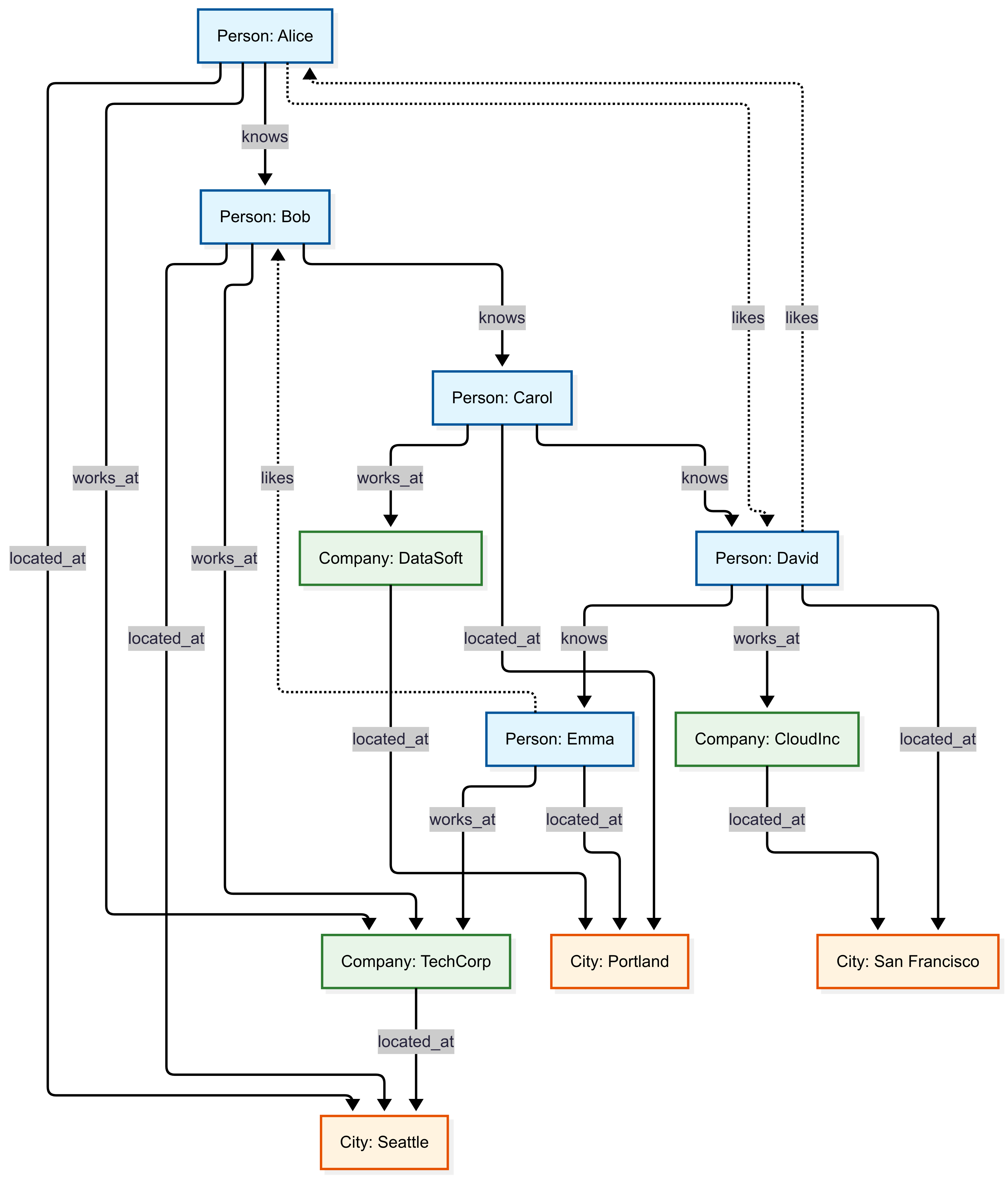
Simple educational graph for learning fundamentals
Usage: graph("Simple")
Purpose: Basic graph operations and learning fundamental graph query patterns.
Description: A small educational graph containing people, companies, and cities with various relationships. Perfect for learning graph traversals and understanding basic patterns. This compact dataset includes 11 nodes (5 people, 3 companies, and 3 cities) connected through 20 relationships, making it ideal for understanding graph fundamentals without the complexity of larger datasets. The graph demonstrates common real-world scenarios like employment relationships, geographic locations, social connections, and personal preferences.
Use Cases:
- Learning graph query fundamentals
- Testing graph algorithms
- Understanding relationship patterns
- Educational examples for graph concepts
Schema Relationships:
Schema and Counts:
Node Types:
Person- Individual people (5 nodes)Company- Business organizations (3 nodes)City- Geographic locations (3 nodes)
Relationship Types:
works_at- Employment relationships (5 edges)located_at- Geographic location assignments (8 edges)knows- Social connections between people (4 edges)likes- Personal preferences and interests (3 edges)
Graph Instance Example:
This example demonstrates basic graph relationships in a small, easy-to-understand network showing how people connect to companies and cities through various relationship types.
Example Queries:
Find all employees of a specific company:
graph("Simple")
| graph-match (person)-[works_at]->(company)
    where company.name == "TechCorp"
    project employee_name = person.name, employee_age = person.properties.age
| employee_name | employee_age |
|---|---|
| Alice | 25 |
| Bob | 30 |
| Emma | 26 |
Find colleagues (people working at the same company):
graph("Simple")
| graph-match (person1)-->(company)<--(person2)
    where person1.id != person2.id and labels(company) has "Company"
    project colleague1 = person1.name, colleague2 = person2.name, company = company.name
| take 1
| colleague1 | colleague2 | company |
|---|---|---|
| Alice | Bob | TechCorp |
LDBC SNB interactive
Usage: graph("LDBC_SNB_Interactive")
Purpose: Social network traversals and friend-of-friend exploration.
Use Cases:
- Social network analysis and recommendation systems
- Community detection algorithms
- Influence propagation studies
- Content recommendation based on social connections
- Friend-of-friend discovery
- Social graph mining research
Graph Schema Overview:
Schema and Counts:
Core Social Entity Types:
PERSON- Social network users (1,528 nodes)POST- User posts (135,701 nodes)COMMENT- Comments on posts (151,043 nodes)FORUM- Discussion forums (13,750 nodes)
Organizational and Geographic Types:
ORGANISATION- Universities and companies (7,955 nodes)PLACE- Geographic locations: continents (6), countries (111), cities (1,343) - total 1,460 nodes
Content Classification Types:
TAG- Content tags (16,080 nodes)TAGCLASS- Tag categories (71 nodes)
Key Relationship Types:
KNOWS- Friend relationships (14,073 edges)LIKES- Content likes: posts (47,215) + comments (62,225) = 109,440 total edgesHAS_CREATOR- Content authorship: posts (135,701) + comments (151,043) = 286,744 edgesHAS_MEMBER- Forum memberships (123,268 edges)HAS_TAG- Content tagging: posts (51,118) + comments (191,303) + forums (47,697) = 290,118 edgesIS_LOCATED_IN- Location relationships: people (1,528) + organizations (7,955) + posts (135,701) + comments (151,043) = 296,227 edgesREPLY_OF- Comment threading: comment-to-comment (76,787) + comment-to-post (74,256) = 151,043 edgesWORK_AT/STUDY_AT- Professional/educational history (4,522 edges)HAS_INTEREST- Personal interests (35,475 edges)- Other relationships:
HAS_MODERATOR,IS_PART_OF,CONTAINER_OF,HAS_TYPE,IS_SUBCLASS_OF
Graph Instance Example:
This example demonstrates complex social network interactions in a realistic social media environment, showing how users engage with content, participate in forums, and form social connections.
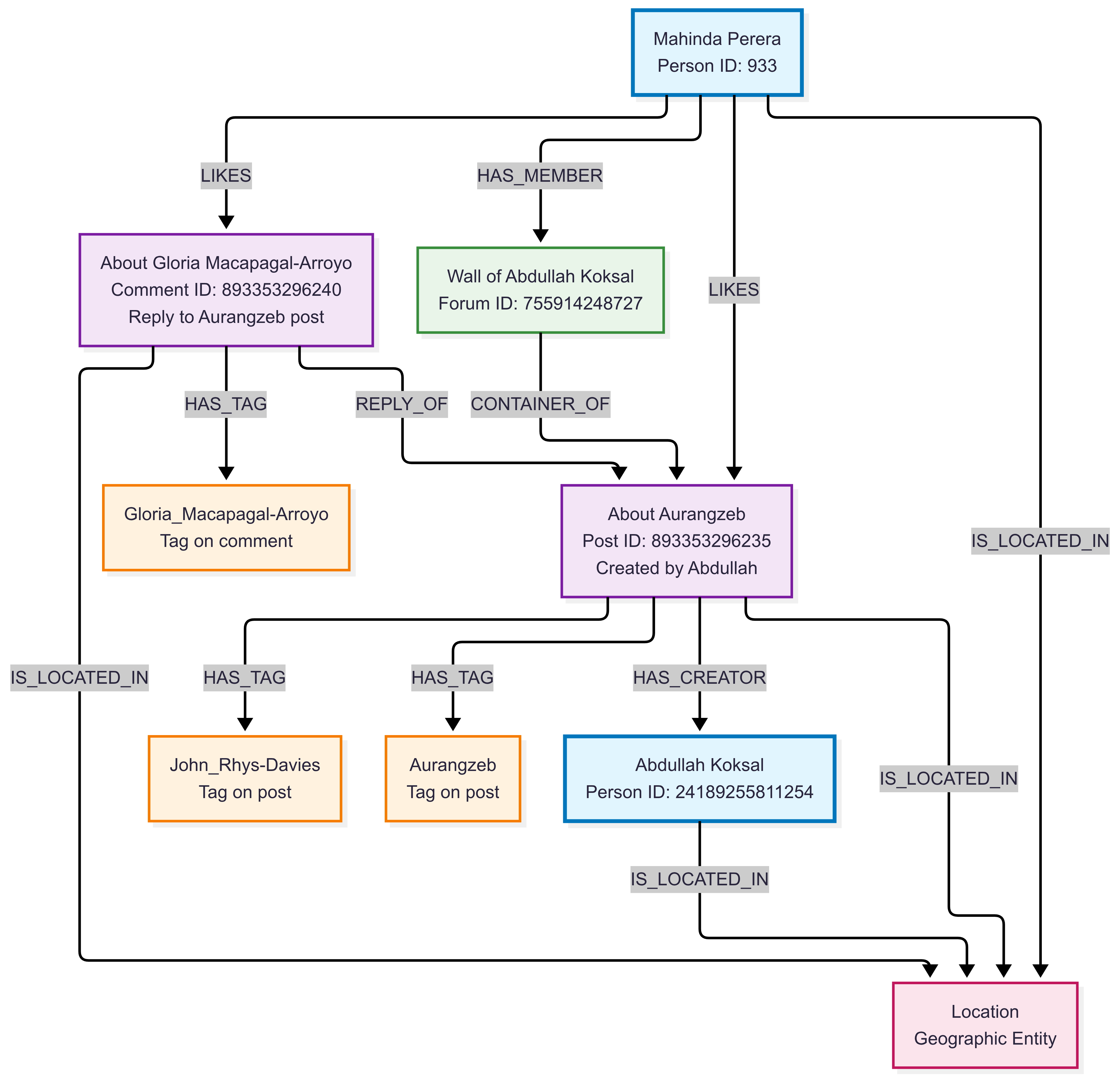
This example demonstrates:
- Social Engagement: Mahinda likes both Abdullah’s post and a comment on that post
- Content Threading: The comment (about Gloria Macapagal-Arroyo) replies to the post (about Aurangzeb)
- Content Creation: Abdullah creates posts in his own forum wall
- Community Participation: Mahinda is a member of Abdullah’s forum where the content appears
- Content Classification: Both posts and comments are tagged with relevant topics from their content
- Geographic Context: All entities have location relationships for geographic analysis
Use Cases:
- Social network analysis and recommendation systems
- Community detection algorithms
- Influence propagation studies
- Content recommendation based on social connections
- Friend-of-friend discovery
- Social graph mining research
Example Queries:
Find direct friendships with similar ages:
graph("LDBC_SNB_Interactive")
| graph-match (person1)-[knows]->(person2)
    where labels(person1) has "PERSON" and labels(person2) has "PERSON" and
        labels(knows) has "KNOWS"and abs(person1.birthday - person2.birthday) < 30d
    project person_name = person1.firstName, friend_name = person2.firstName
| count
| Count |
|---|
| 225 |
Find popular posts by likes:
This query analyzes social engagement by identifying the most popular content creators based on how many unique people have liked their posts. It traverses the social network graph through the path: person → likes → post → has_creator → creator. The query aggregates the data to show each creator’s total number of unique likers and distinct posts, then returns the top 3 creators with the most likes. This is useful for identifying influential content creators, understanding engagement patterns, and discovering viral content in the social network.
graph("LDBC_SNB_Interactive")
| graph-match (person)-[likes]->(post)-[has_creator]->(creator)
    where labels(person) has "Person" and labels( post) has "POST" and labels(has_creator) has "HAS_CREATOR" and isnotempty(creator.lastName)
    project personId = person.id, postId = post.id, creator = creator.lastName
| summarize Likes = dcount(personId), posts = dcount(postId) by creator
| top 3 by Likes desc
| creator | Likes | posts |
|---|---|---|
| Zhang | 371 | 207 |
| Hoffmann | 340 | 9 |
| Singh | 338 | 268 |
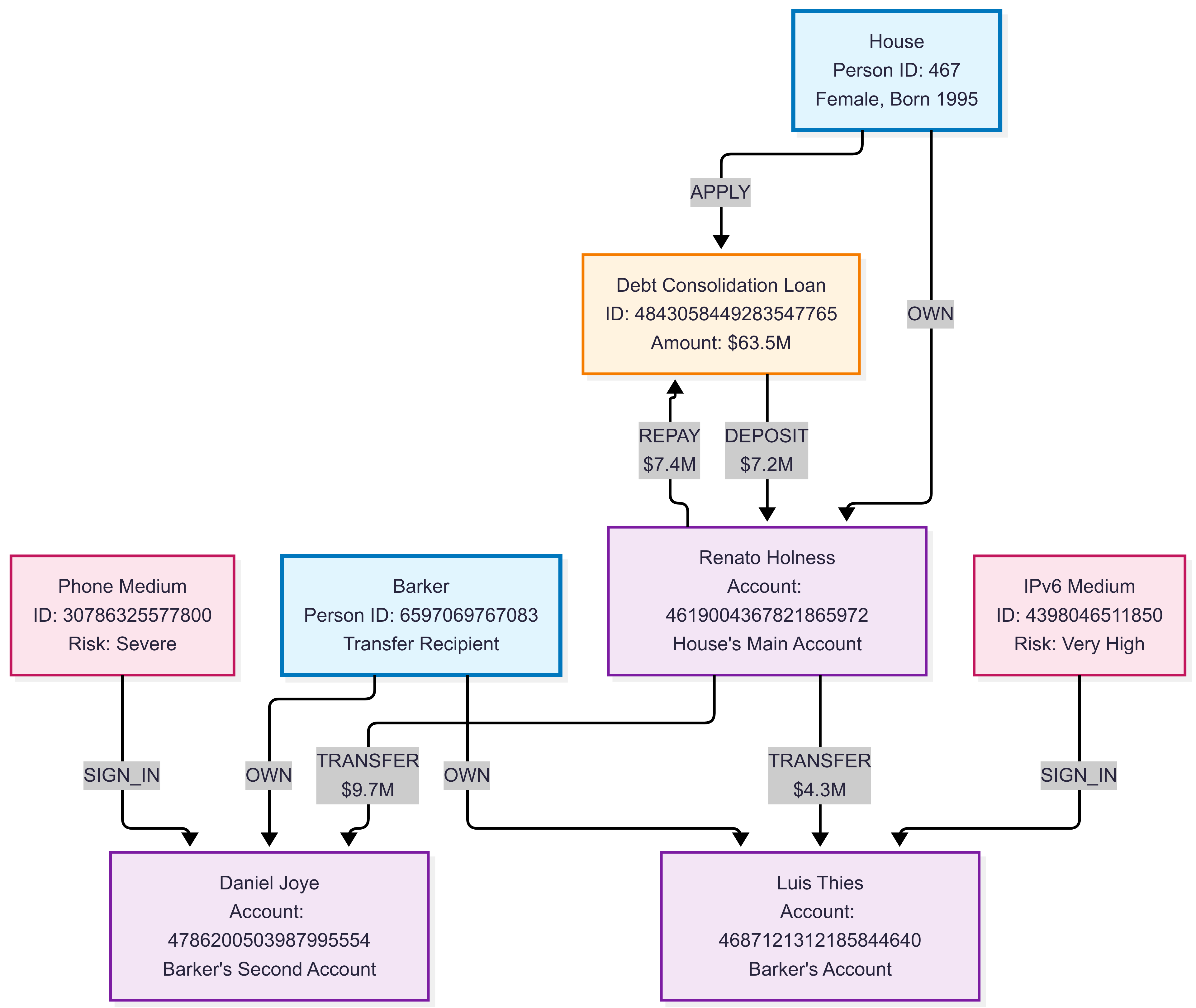
LDBC Financial
Usage: graph("LDBC_Financial")
Purpose: Financial transaction analysis and fraud detection patterns.
Description: LDBC Financial Benchmark dataset representing a comprehensive financial network with companies, persons, accounts, loans, and various financial transactions. This dataset models realistic financial ecosystems with 5,580 total nodes and over 31,000 financial transactions and relationships. Designed specifically for fraud detection, anti-money laundering (AML) analysis, and financial crime investigation scenarios, it captures complex patterns including account ownership, loan applications, guarantees, and multi-step transaction chains that are common in financial crime scenarios.
Use Cases:
- Financial fraud detection
- Anti-money laundering (AML) analysis
- Transaction pattern analysis
- Risk assessment and credit scoring
- Suspicious activity monitoring
- Financial network analysis
Graph Schema Overview:
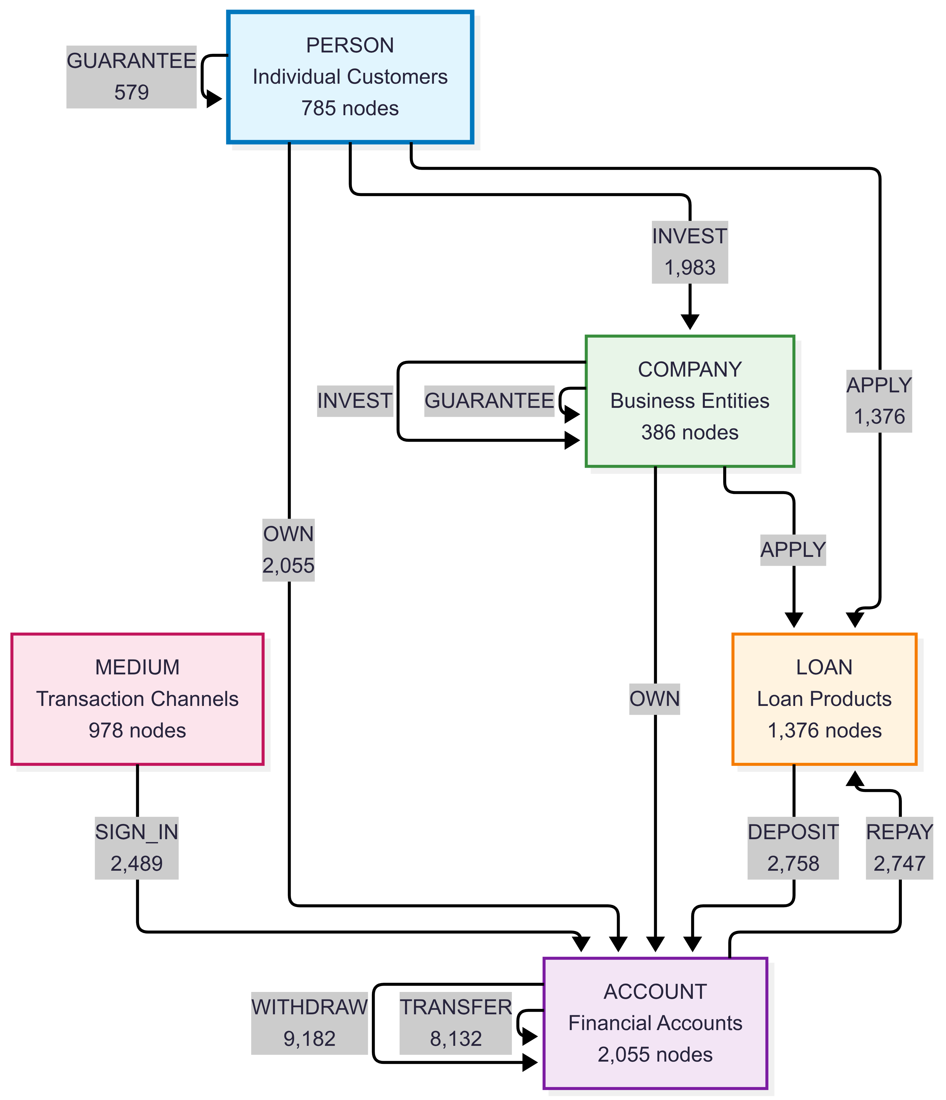
Schema and Counts:
Node Types:
COMPANY- Business entities (386 nodes)PERSON- Individual customers (785 nodes)ACCOUNT- Financial accounts (2,055 nodes)LOAN- Loan products (1,376 nodes)MEDIUM- Transaction mediums/channels (978 nodes)
Relationship Types:
TRANSFER- Money transfers between accounts (8,132 edges)WITHDRAW- Cash withdrawals from accounts (9,182 edges)DEPOSIT- Money deposits into accounts (2,758 edges)OWN- Account ownership relationships (2,055 edges)APPLY- Loan applications (1,376 edges)GUARANTEE- Loan guarantees (579 edges)INVEST- Investment transactions (1,983 edges)REPAY- Loan repayments (2,747 edges)SIGN_IN- Authentication events (2,489 edges)
Graph Instance Example:
This example illustrates a complex financial network with multiple entity types and transaction patterns, demonstrating how financial institutions can model relationships between customers, accounts, loans, and transaction flows for fraud detection and risk assessment.
Example Queries:
Detect potential money laundering through circular transfers:
This query identifies suspicious circular transaction patterns that could indicate money laundering activities. It searches for accounts that send money to another account and then receive it back through a chain of 1 to 3 transfers, creating a circular flow. The query specifically looks for large initial transfers (over 10,000) and returns details about the suspicious accounts, including the transfer amount and the length of the circular chain. This pattern detection is useful for anti-money laundering (AML) systems and financial fraud investigations.
graph("LDBC_Financial")
| graph-match (account1)-[t1]->(account2)-[t2*1..3]->(account1)
    where labels(t1) has "TRANSFER" and t1.amount > 10000  // Large initial transfer
    project suspicious_account = account1.node_id,
            amount = t1.amount,
            transfer_chain_length = array_length(t2) + 1
| take 10
| suspicious_account | amount | transfer_chain_length |
|---|---|---|
| Account::4818007176356300028 | 5035377,73 | 2 |
| Account::4818007176356300028 | 5035377,73 | 2 |
| Account::4845310249097233848 | 359062,45 | 2 |
| Account::4818007176356300028 | 5035377,73 | 3 |
| Account::4818007176356300028 | 5035377,73 | 4 |
| Account::4840243699516440940 | 5753668,55 | 4 |
| Account::4818007176356300028 | 5035377,73 | 4 |
| Account::180143985094820389 | 465338,26 | 4 |
| Account::4814910951612482356 | 1684581,62 | 4 |
| Account::4816599801472746629 | 963626,42 | 4 |
Find high-risk loan guarantors:
This query identifies individuals or companies who guarantee multiple loans totaling significant amounts, which could indicate financial risk exposure. It traverses the financial network graph following the path: guarantor → guarantee → borrower → apply → loan. The query aggregates the total amount guaranteed and number of loans for each guarantor, then filters for those guaranteeing over 100,000 in total and returns the top 5 by total guaranteed amount. This analysis is useful for risk assessment, identifying over-leveraged guarantors, and evaluating systemic financial risks in lending networks.
graph("LDBC_Financial")
| graph-match (guarantor)-[guarantee]->(borrower)-[apply]->(loan)
    where labels(guarantee) has "GUARANTEE" and labels(apply) has "APPLY"
    project guarantor_id = guarantor.node_id,
            borrower_id = borrower.node_id,
            loan_amount = loan.loanAmount
| summarize total_guaranteed = sum(loan_amount), loan_count = count() by guarantor_id
| where total_guaranteed > 100000
| top 5 by total_guaranteed desc
| guarantor_id | total_guaranteed | loan_count |
|---|---|---|
| Person::44 | 439802195 | 8 |
| Person::15393162789155 | 411111642 | 8 |
| Company::12094627905931 | 404538891 | 6 |
| Company::4398046511208 | 366243272 | 8 |
| Person::19791209300551 | 338838223 | 6 |
BloodHound Entra dataset
Usage: graph("BloodHound_Entra")
Purpose: Microsoft Entra privilege escalation and attack path analysis.
Description: BloodHound dataset for Microsoft Entra environments. This comprehensive security dataset contains 13,526 Microsoft Entra objects including users, groups, applications, service principals, devices, and various cloud resources. With over 800,000 permission relationships and security edges, it models complex Microsoft Entra environments typical of enterprise organizations. The dataset captures detailed Microsoft Entra permissions, role assignments, group memberships, and resource ownership patterns essential for identifying privilege escalation paths and attack vectors in cloud environments.
Use Cases:
- Entra ID security assessments
- Privilege escalation path discovery
- Attack path visualization
- Identity governance analysis
- Risk-based security controls
- Compliance auditing for cloud environments
Graph Schema Overview:
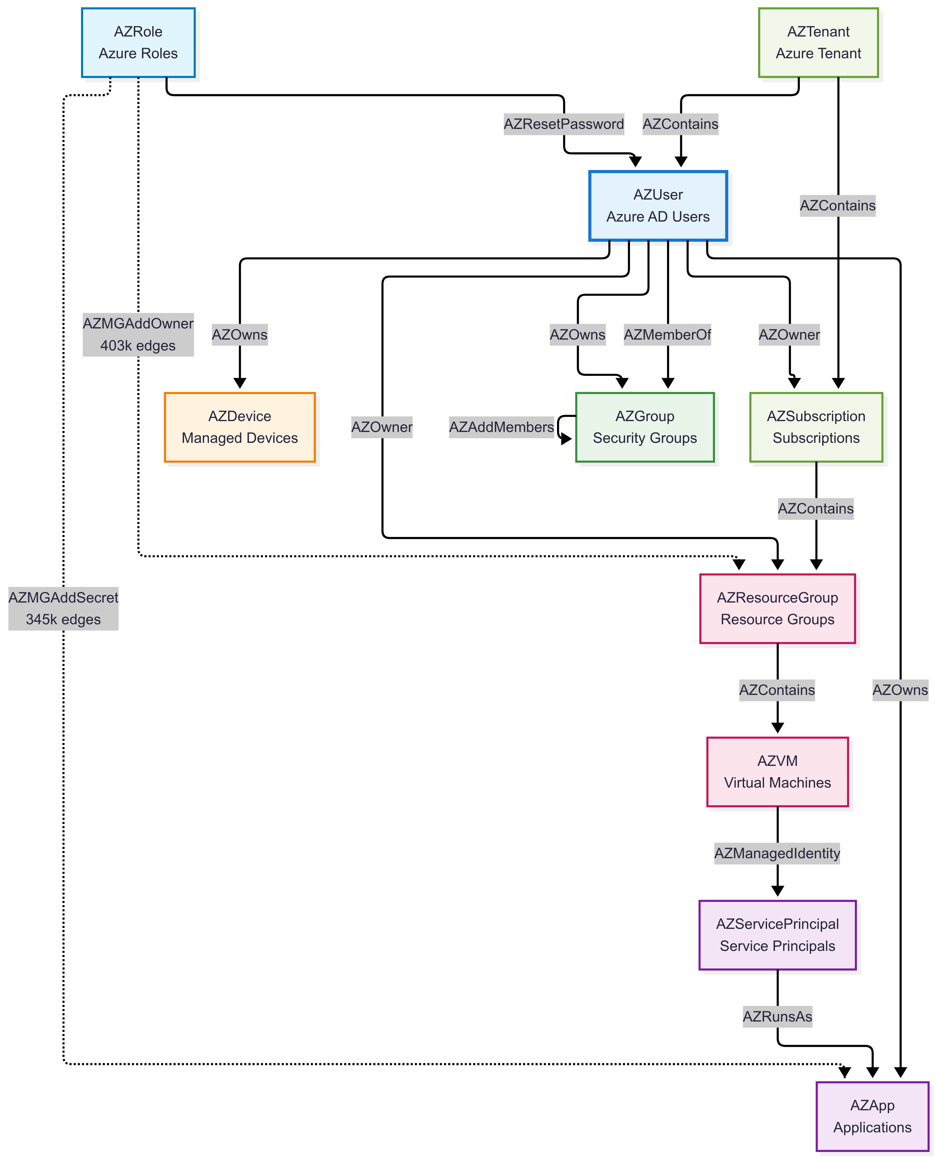
Schema and Counts:
Description: BloodHound Community Edition dataset for Microsoft Entra environments. This comprehensive security dataset contains 13,526 Microsoft Entra objects including users, groups, applications, service principals, devices, and various cloud resources. With over 800,000 permission relationships and security edges, it models complex Microsoft Entra environments typical of enterprise organizations. The dataset captures detailed Microsoft Entra permissions, role assignments, group memberships, and resource ownership patterns essential for identifying privilege escalation paths and attack vectors in cloud environments.
Schema and Counts:
Primary Node Types:
AZUser- Microsoft Entra users (230 nodes)AZServicePrincipal- Service principals and applications (6,270 nodes)AZApp- Azure applications (6,648 nodes)AZGroup- Microsoft Entra groups (58 nodes)AZDevice- Managed devices (47 nodes)
Azure Resource Types:
AZResourceGroup- Resource groups (59 nodes)AZVM- Virtual machines (66 nodes)AZRole- Azure roles (116 nodes)AZSubscription- Azure subscriptions (3 nodes)AZTenant- Azure tenant (1 node)
Key Relationship Types (Top permissions by volume):
AZMGAddOwner- Management group owner permissions (403,412 edges)AZMGAddSecret- Secret management permissions (345,324 edges)AZAddSecret- Application secret permissions (24,666 edges)AZContains- Resource containment relationships (12,924 edges)AZRunsAs- Service execution permissions (6,269 edges)AZMemberOf- Group membership relationships (4,439 edges)AZOwns- Resource ownership (2,870 edges)
Graph Instance Example:
This example demonstrates Microsoft Entra and Entra identity relationships with complex privilege structures and potential attack paths in a cloud environment.
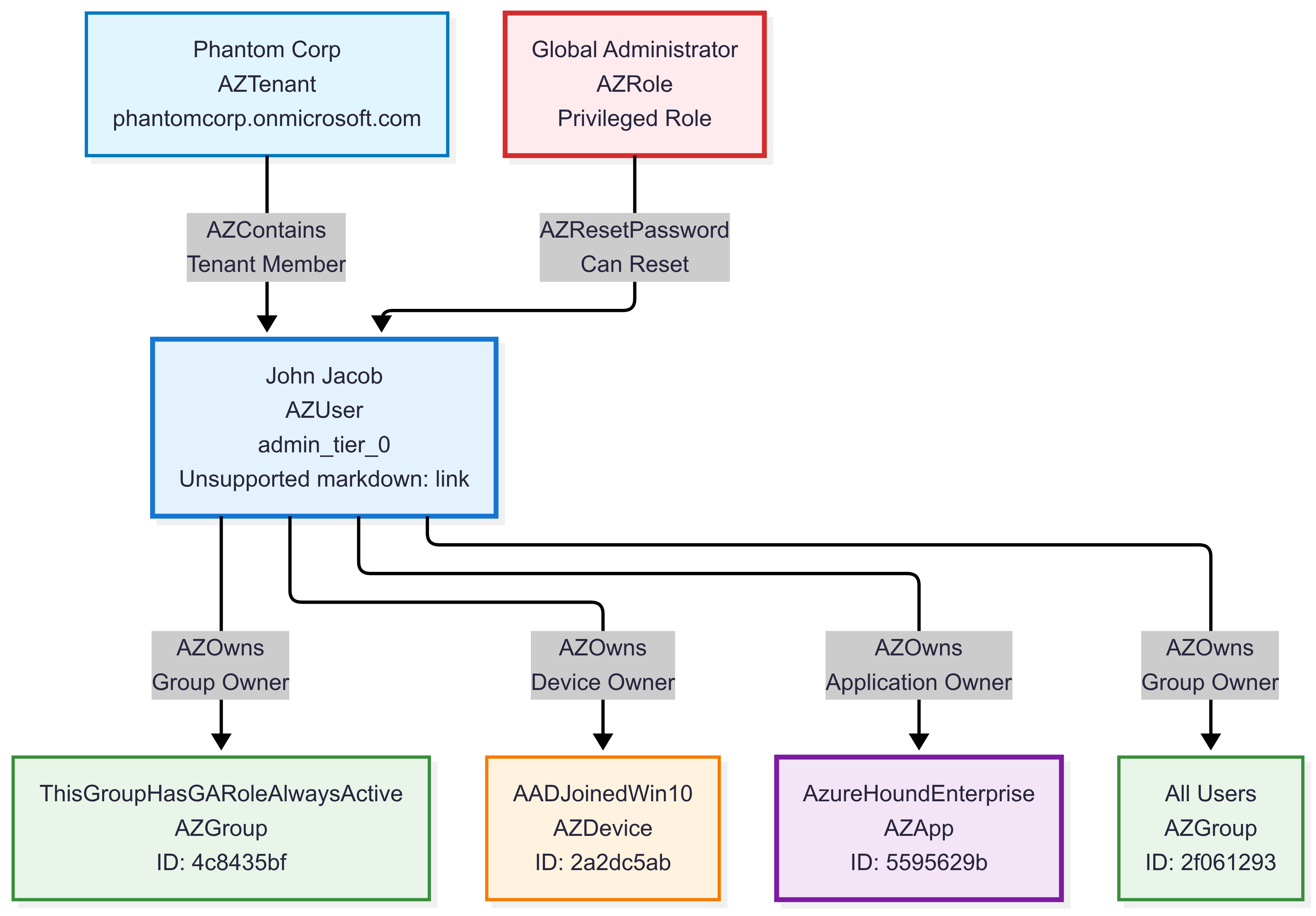
Use Cases:
- Entra ID security assessments
- Privilege escalation path discovery
- Attack path visualization
- Identity governance analysis
- Risk-based security controls
- Compliance auditing for cloud environments
Example Queries:
Find paths to administrative privileges:
This query identifies privilege escalation paths from regular users to administrative groups in Microsoft Entra environments. It searches for users who can reach admin groups (like Microsoft Entra DC Administrators, DnsAdmins, etc.) through 1-3 relationship hops, helping security teams understand potential attack paths and privilege escalation risks.
graph("BloodHound_Entra")
| graph-match (user)-[path*1..3]->(admingroup)
    where labels(user) has_any ("User", "AZUser")
          and labels(admingroup) has_any ("Group", "AZGroup")
          and (admingroup.name contains "ADMIN" or admingroup.displayname contains "ADMIN")
    project source_user = user.name,
             path_length = array_length(path),
             admin_group = coalesce(admingroup.displayname, admingroup.name)
| take 10
| source_user | path_length | admin_group |
|---|---|---|
| THISUSERHASINTUNEADMINROLE@PHANTOMCORP.ONMICROSOFT.COM | 1 | ADSyncAdmins |
| 097EF6C2-GROUPSADMINISTRATOR@PHANTOMCORP.ONMICROSOFT.COM | 1 | AAD DC Administrators |
| USERBELONGSTOGAGROUP@PHANTOMCORP.ONMICROSOFT.COM | 1 | ADSyncAdmins |
| THISUSERHASINTUNEADMINROLE@PHANTOMCORP.ONMICROSOFT.COM | 1 | DnsAdmins |
| RHADMIN@PHANTOMCORP.ONMICROSOFT.COM | 1 | DnsAdmins |
| CJACKSON@PHANTOMCORP.ONMICROSOFT.COM | 1 | Azure ATP phantom Administrators |
| 097EF6C2-INTUNEADMINISTRATOR@PHANTOMCORP.ONMICROSOFT.COM | 1 | AAD DC Administrators |
| RHADMIN_PHANTOMCORP.ONMICROSOFT.COM#EXT#@PHANTOMCORP.ONMICROSOFT.COM | 1 | Resource Group Admins |
| THISUSERHASKNOWLEDGEMANAGERROLE@PHANTOMCORP.ONMICROSOFT.COM | 1 | DnsAdmins |
| 097EF6C2-INTUNEADMINISTRATOR@PHANTOMCORP.ONMICROSOFT.COM | 1 | DnsAdmins |
Identify high-value targets (Tier 0 assets):
This query identifies critical administrative assets marked as “admin_tier_0” in the environment. These are the most sensitive and powerful accounts, service principals, and resources that pose the highest risk if compromised. Understanding these assets helps prioritize security monitoring and protection efforts.
graph("BloodHound_Entra")
| graph-match (asset)
    where asset.properties.system_tags contains "admin_tier_0"
    project asset_name = asset.name,
             asset_type = tostring(labels(asset)[1]),  // Get primary type (AZUser, AZServicePrincipal, etc.)
             system_tags = asset.properties.system_tags
| take 10
| asset_name | asset_type | system_tags |
|---|---|---|
| JJACOB@PHANTOMCORP.ONMICROSOFT.COM | AZUser | admin_tier_0 |
| PLEWIS@PHANTOMCORP.ONMICROSOFT.COM | AZUser | admin_tier_0 |
| JMILLER@PHANTOMCORP.ONMICROSOFT.COM | AZUser | admin_tier_0 |
| CJACKSON@PHANTOMCORP.ONMICROSOFT.COM | AZUser | admin_tier_0 |
| RHALL@PHANTOMCORP.ONMICROSOFT.COM | AZUser | admin_tier_0 |
| THISAPPHASGLOBALADMIN@PHANTOMCORP | AZServicePrincipal | admin_tier_0 |
| MYCOOLAUTOMATIONACCOUNT@PHANTOMCORP | AZServicePrincipal | admin_tier_0 |
| SERVICEPRINCIPALE@PHANTOMCORP | AZServicePrincipal | admin_tier_0 |
| 31E3B75F-PRIVILEGED AUTHENTICATION ADMINISTRATOR@PHANTOMCORP | AZServicePrincipal | admin_tier_0 |
| 31E3B75F-PRIVILEGED ROLE ADMINISTRATOR@PHANTOMCORP | AZServicePrincipal | admin_tier_0 |
BloodHound Active Directory dataset
Usage: graph("BloodHound_AD")
Purpose: On-premises Active Directory security analysis and privilege mapping.
Description: BloodHound Community Edition dataset for on-premises Active Directory environments. This dataset contains 1,495 Active Directory objects representing a typical enterprise AD deployment with complex permission structures and attack paths. The dataset includes users, computers, groups, organizational units, group policy objects, and certificate authority components across multiple domains. With over 18,000 permission relationships and security edges, it captures realistic AD attack scenarios including privilege escalation paths, ACL-based permissions, group memberships, and certificate-based authentication vulnerabilities common in Windows domain environments.
Use Cases:
- Active Directory security assessments
- Attack path analysis and penetration testing
- Domain privilege mapping
- Group policy security analysis
- Kerberoasting and ASREPRoasting target identification
- Security control gap analysis
Graph Schema Overview:
Core AD Object Types:
User- Domain users (99 nodes)Computer- Domain computers (34 nodes)Group- Security and distribution groups (219 nodes)ADLocalGroup- Local groups on computers (28 nodes)GPO- Group Policy Objects (32 nodes)
AD Infrastructure Types:
Domain- Active Directory domains (5 nodes)OU- Organizational Units (20 nodes)Container- AD containers (939 nodes)CertTemplate- Certificate templates (106 nodes)EnterpriseCA- Certificate Authorities (4 nodes)RootCA- Root Certificate Authorities (5 nodes)
Key Permission Types (Top attack vectors):
GenericAll- Full control permissions (3,292 edges)WriteDacl- Modify permissions (2,221 edges)WriteOwner- Change ownership (2,187 edges)Owns- Object ownership (1,439 edges)Contains- Containment relationships (1,416 edges)GenericWrite- Write permissions (579 edges)MemberOf- Group memberships (301 edges)
Graph Schema Overview:
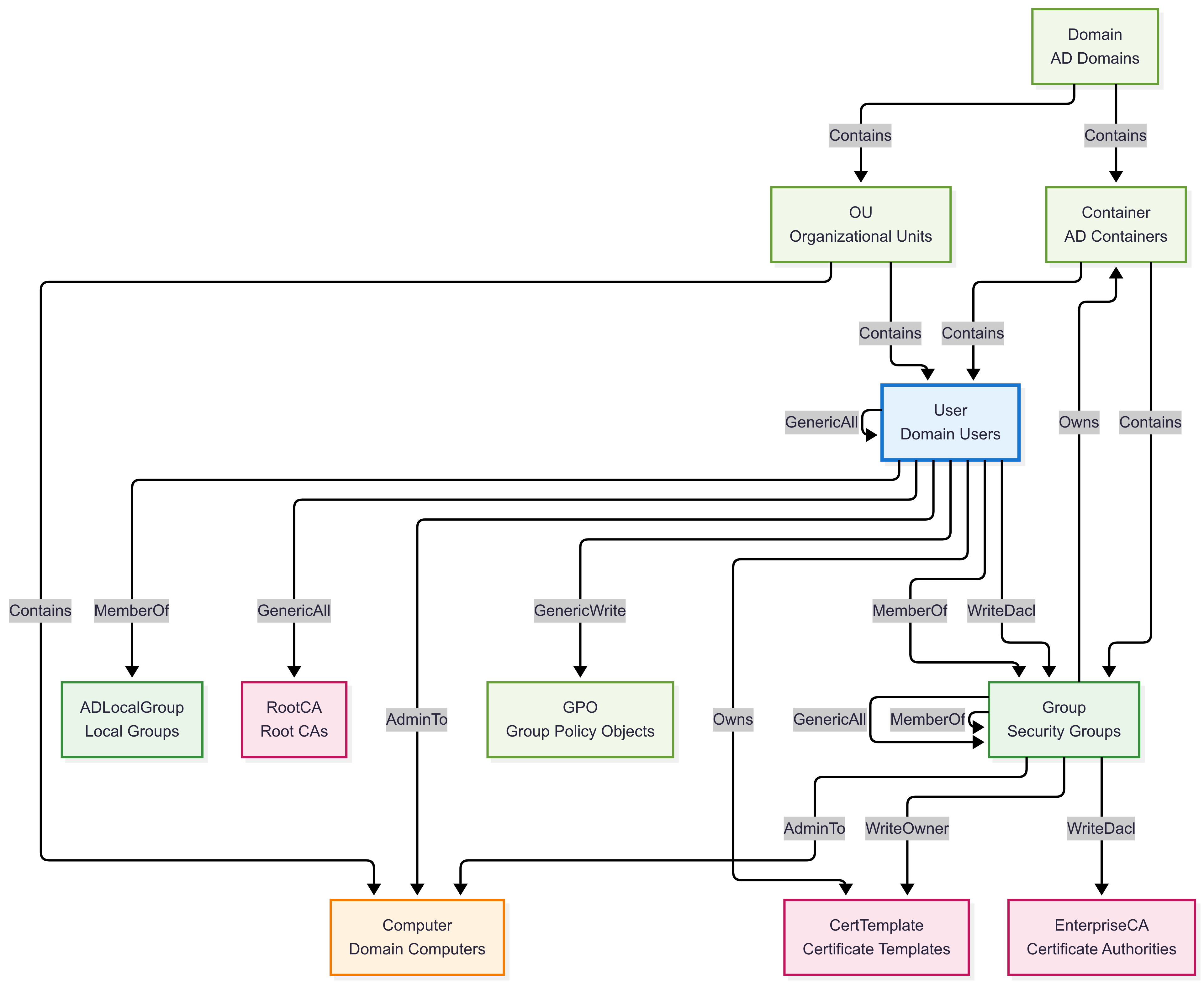
Graph Instance Example:
This example demonstrates on-premises Active Directory attack paths and potential security vulnerabilities in a traditional Windows domain environment.
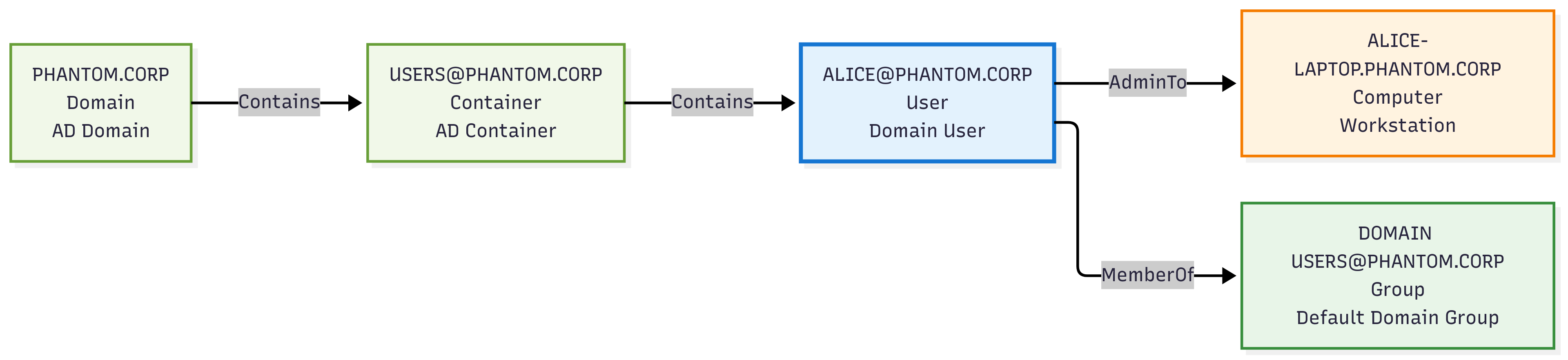
Use Cases:
- Active Directory security assessments
- Attack path analysis and penetration testing
- Domain privilege mapping
- Group policy security analysis
- Kerberoasting and ASREPRoasting target identification
- Security control gap analysis
Example Queries:
Find potential privilege escalation:
This query counts how many non-admin users can potentially escalate to admin in Microsoft Entra. It traverses up to 10 MemberOf group hops (no cycles) from each user to groups that grant dangerous permissions (GenericAll, WriteDacl, WriteOwner, ForceChangePassword) over admin users (admincount=true), then returns the distinct number of such “potential attacker” users.
graph("BloodHound_AD")
| graph-match cycles=none (user)-[memberof*0..10]->(group)-[permission]->(target)
    where labels(user) has "User"
          and labels(group) has "Group"
          and all(memberof, labels() has "MemberOf")
          and user.properties.admincount == false
          and (labels(permission) has_any ("GenericAll", "WriteDacl", "WriteOwner", "ForceChangePassword"))
          and (labels(target) has "User" and target.properties.admincount == true)
    project  attack_user = user.name
| summarize ['Potential attackers'] = dcount(attack_user)
| Potential attackers |
|---|
| 2 |
Find Golden Certificate attack paths:
This query identifies entities that can perform Golden Certificate attacks, which allow attackers to forge certificates as any user in the domain. These are critical vulnerabilities as they enable complete domain compromise by allowing the attacker to impersonate any user, including domain administrators, through forged certificates.
graph("BloodHound_AD")
| graph-match (attacker)-[goldencert]->(target)
    where labels(goldencert) has "GoldenCert"
    project
        Attacker = attacker.name,
        AttackerType = case(
            attacker.name has "DC", "Domain Controller",
            attacker.name has "CA", "Certificate Authority",
            attacker.name has "SRV", "Server",
            "Unknown System"
        ),
        Target = target.name,
        RiskLevel = "CRITICAL",
        AttackCapability = case(
            attacker.name has "DC", "Primary domain controller with certificate services",
            attacker.name has "EXTCA", "External Certificate Authority with root access",
            attacker.name has "SRV", "Compromised server with certificate generation rights",
            "System with certificate forging capabilities"
        )
| Attacker | AttackerType | Target | RiskLevel | AttackCapability |
|---|---|---|---|---|
| DC01.PHANTOM.CORP | Unknown System | PHANTOM.CORP | CRITICAL | System with certificate forging capabilities |
| SRV-SHARPHOUND.PHANTOM.CORP | Server | PHANTOM.CORP | CRITICAL | Compromised server with certificate generation rights |
| EXTCA01.WRAITH.CORP | Unknown System | WRAITH.CORP | CRITICAL | System with certificate forging capabilities |
| EXTCA02.WRAITH.CORP | Unknown System | WRAITH.CORP | CRITICAL | System with certificate forging capabilities |
Related content
5 - Graph semantics overview
Graph semantics enables you to model and query data as interconnected networks. A graph consists of nodes (entities) and edges (relationships) that connect them. Both nodes and edges can contain properties, creating a rich data model for complex relationships.
Graphs excel at representing complex data with many-to-many relationships, hierarchical structures, or networked connections—such as social networks, recommendation systems, connected assets, and knowledge graphs. Unlike relational databases that require indexes and joins to connect data across tables, graphs use direct adjacency between nodes, enabling fast and intuitive traversal of relationships.
The following graph illustrates a cybersecurity attack path scenario. Nodes represent entities such as external sources, users, and critical assets, while edges represent actions or relationships that form a potential attack sequence.
Graph queries leverage graph structure to perform sophisticated operations such as finding paths, patterns, shortest distances, communities, and centrality measures. These capabilities make graphs powerful for modeling relationships, interactions, dependencies, and flows across domains—including social networks, supply chains, IoT device networks, digital twins, recommendation systems, and organizational structures.
The following graph shows a supply chain scenario where nodes represent suppliers, manufacturers, and distributors, and edges represent supply relationships. This example demonstrates how graphs model flows and dependencies across different business contexts.
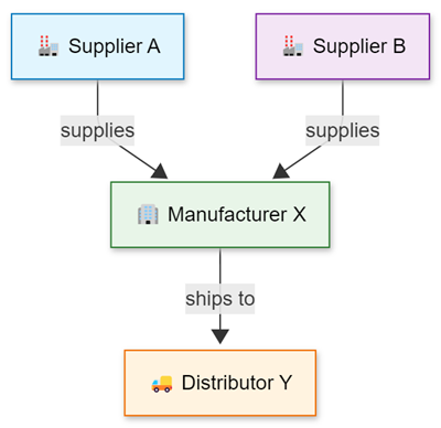
Why use graph semantics?
Graph capabilities offer significant advantages by leveraging existing data investments while adding sophisticated relationship modeling:
- No data migration required - Build graph models directly from current data without duplication.
- Cost-effective solution - Eliminates the complexity and expense of dedicated graph databases.
- Temporal analysis support - As a time-series database, you can naturally analyze how graphs evolve over time.
- Event-based modeling - Models graphs as sequences of relationship events, aligning with strong event processing capabilities.
- Seamless KQL integration - Graph operators work alongside all existing KQL capabilities with full IntelliSense support.
This approach delivers enterprise-grade relationship modeling while maintaining performance, scale, and a familiar interface. Organizations can analyze complex interconnected data across domains—from supply chains and organizational hierarchies to IoT device networks and social relationships—without extra infrastructure investments.
Transient graph creation approach
Transient graphs are created dynamically using the make-graph operator. These graphs exist in memory during query execution and are automatically discarded when the query completes.
Key characteristics
- Dynamic creation - Built from tabular data using KQL queries with the entire structure residing in memory
- Immediate availability - No preprocessing or setup requirements
- Memory constraints - Graph size is limited by available memory on cluster nodes
- Performance factors - Graph topology and property sizes determine memory requirements
This approach is optimal for smaller to medium-sized datasets where immediate analysis is needed.
Use cases for transient graphs
Transient graphs excel in several scenarios:
- Ad hoc analysis - One-time investigations requiring quick pattern examination
- Exploratory data analysis - Testing hypotheses and validating analytical approaches
- Small to medium datasets - Real-time analysis of recent events or focused data subsets
- Rapid prototyping - Testing graph patterns before implementing persistent models
- Dynamic data analysis - Frequently changing data that doesn’t justify persistent storage
Common applications include real-time IoT monitoring, supply chain relationship analysis, customer journey mapping, and any scenario requiring immediate visualization of entity relationships.
Persistent graph creation approach
Persistent graphs use graph models and graph snapshots to provide robust solutions for large-scale, complex graphs representing organizational networks, supply chains, IoT ecosystems, digital twins, and other interconnected data domains.
Key characteristics for persistent graphs
- Persistent storage - Graph models and snapshots are stored in database metadata for durability and consistency
- Scalability - Handle graphs exceeding memory limitations with enterprise-scale analysis capabilities
- Reusability - Multiple users can query the same structure without rebuilding, enabling collaborative analysis
- Performance optimization - Eliminate graph construction latency for repeated queries
- Version control - Multiple snapshots represent graphs at different time points for historical analysis
- Schema support - Structured definitions for different entity types and their properties
The schema capability supports both static labels (predefined in the graph model) and dynamic labels (generated at runtime from data), providing flexibility for complex environments with diverse entity types.
Use cases for persistent graphs
Persistent graphs are essential for:
- Enterprise analytics - Continuous monitoring workflows across complex networks
- Large-scale data analysis - Enterprise-scale graphs with millions of nodes and relationships
- Collaborative analysis - Multiple teams working with shared graph structures
- Production workflows - Automated systems requiring consistent graph access
- Historical comparison - Time-based analysis of graph evolution and changes
Example: Digital Twin Persistent Graph
In digital twin and IoT scenarios, persistent graphs support regular analysis of device relationships, equipment dependencies, and system evolution over time. Historical analysis allows comparing system states across different periods, tracking the evolution of assets, and conducting long-term trend analysis.
Example: IoT and digital twin persistent graph
- Create comprehensive models of IoT deployments and connected assets
- Support real-time monitoring, predictive maintenance, and performance optimization
- Analyze equipment dependencies and identify potential failure points
- Optimize sensor placements through physical and logical topology understanding
- Track device configurations, communications, and performance characteristics over time
- Detect communication pattern anomalies and visualize smart environment evolution
- Simulate operating conditions before implementing physical infrastructure changes
This persistent approach proves invaluable for managing complex IoT ecosystems at scale.
Graph querying capabilities
Once a graph is established (through make-graph or from a snapshot), you can leverage the full suite of KQL graph operators for comprehensive analysis:
Core operators:
graph-match- Enables sophisticated pattern matching and traversal operations for identifying complex relationship sequencesgraph-shortest-paths- Finds optimal paths between entities, helping prioritize connections and identify critical relationshipsgraph-to-table- Converts graph analysis results to tabular format for integration with existing systems
Advanced analysis capabilities:
- Time-based analysis - Examine how relationships and patterns evolve over time
- Geospatial integration - Combine graph data with location-based intelligence for geographic pattern analysis
- Machine learning integration - Apply algorithms for entity clustering, pattern classification, and anomaly detection
These capabilities support diverse use cases including customer journey analysis, product recommendation systems, IoT networks, digital twins, and knowledge graphs.
Choosing the right approach
The following decision tree helps you select the most appropriate graph creation approach based on your specific requirements and constraints.
Decision Tree: Transient vs Persistent Graphs
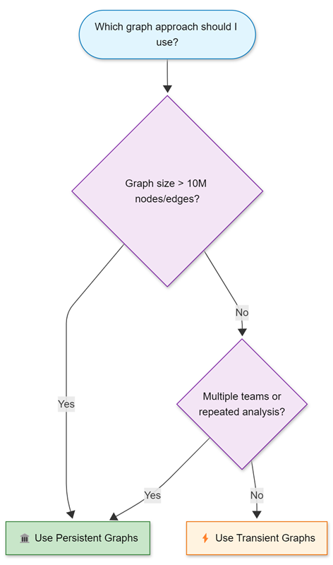
When to use transient graphs
Choose transient graphs for:
- Graph size under 10 million nodes and edges (for optimal performance)
- Single user or small team analysis with minimal collaboration requirements
- One-time or exploratory investigations where immediate results are needed
- Real-time data analysis requiring current state information
- Rapid prototyping and testing of graph patterns and query logic
While transient graphs can handle larger datasets, query execution time increases as the graph must be reconstructed for every query. Consider this performance trade-off when working with larger datasets.
When to use persistent graphs
Choose persistent graphs for:
- Graph size exceeding 10 million nodes and edges where distributed storage is beneficial
- Multiple teams requiring shared access for collaborative analysis
- Repeated analysis on stable datasets where construction latency impacts productivity
- Production workflow integration requiring consistent, reliable graph access
- Historical comparison requirements for tracking changes over time
- Memory capacity limitations affecting query performance
- Collaborative investigation workflows across teams and time zones
Persistent graphs are essential when working with enterprise-scale data or when memory limitations affect performance.
Performance considerations
Memory usage
- Transient graphs - Limited by single cluster node memory, constraining use to datasets within available RAM
- Persistent graphs - Leverage distributed storage and optimized access patterns for enterprise-scale data
Query latency
- Transient graphs - Include construction time in each query, with delays increasing for large datasets or external data sources
- Persistent graphs - Eliminate construction latency through prebuilt snapshots, enabling rapid analysis
External data source dependencies, such as cross cluster queries or external tables to SQL and CosmosDB, can significantly affect transient graph construction time because each query must wait for external responses.
Data freshness
- Transient graphs - Always reflect current data state, ideal for real-time analysis
- Persistent graphs - Reflect data at snapshot creation time, providing consistency for collaborative analysis but requiring periodic refreshes
Integration with KQL ecosystem
Graph semantics integrate seamlessly with KQL’s broader capabilities:
- Time-series analysis - Track relationship evolution over time
- Geospatial functions - Analyze location-based patterns and geographic anomalies
- Machine learning operators - Detect patterns, classify behaviors, and identify anomalies
- Scalar and tabular operators - Enable complex transformations, aggregations, and data enrichment
This integration enables sophisticated workflows including supply chain evolution tracking, geographical asset distribution analysis, community detection through clustering algorithms, and correlation of graph insights with traditional log analysis and external intelligence.
Related content
6 - Operators
6.1 - Graph operators
Graph operators enable graph analysis of data by representing tabular data as a graph with nodes and edges, or by referencing persistent graph entities. This setup lets you use graph operations to study the connections and relationships between different data points.
Graph analysis can be performed using either transient graphs (created dynamically from tabular data using make-graph) or persistent graphs (referenced using the graph function). Once a graph is established, you can use graph operators such as graph-match, graph-shortest-paths, and graph-to-table to analyze relationships, find patterns, and transform results back into tabular form for further processing.
Supported graph operators
The following table describes the supported graph operators.
| Operator | Description |
|---|---|
| make-graph | Builds a graph from tabular data. |
| graph | References a persisted graph entity and retrieves the latest or a specific snapshot. |
| graph-match | Searches for patterns in a graph. |
| graph-to-table | Builds nodes or edges tables from a graph. |
| graph-shortest-paths | Finds the shortest paths from a given set of source nodes to a set of target nodes. |
| graph-mark-components | Finds and marks all connected components. |
Related content
6.2 - graph-mark-components operator (preview)
The graph-mark-components operator finds all connected components of a graph and marks each node with a component identifier.
Syntax
G | graph-mark-components [kind = Kind] [with_component_id = ComponentId]
Parameters
| Name | Type | Required | Description |
|---|---|---|---|
| G | string | ✔️ | The graph source. |
| Kind | string | The connected component kind, either weak (default) or strong. A weak component is a set of nodes connected by a path, ignoring the direction of edges. A strong component is a set of nodes connected in both directions, considering the edges’ directions. | |
| ComponentId | string | The property name that denotes the component identifier. The default property name is ComponentId. |
Returns
The graph-mark-components operator returns a graph result, where each node has a component identifier in the ComponentId property. The identifier is a zero-based consecutive index of the components. Each component index is chosen arbitrarily and might not be consistent across runs.
Examples
The following example creates a graph from a set of child-parent pairs and identifies connected components using a family identifier.
let ChildOf = datatable(child:string, parent:string)
[
  "Alice", "Bob",
  "Carol", "Alice",
  "Carol", "Dave",
  "Greg", "Alice",
  "Greg", "Dave",
  "Howard", "Alice",
  "Howard", "Dave",
  "Eve", "Frank",
  "Frank", "Mallory",
  "Eve", "Kirk",
];
ChildOf
| make-graph child --> parent with_node_id=name
| graph-mark-components with_component_id = family
| graph-to-table nodes
Output
| name | family |
|---|---|
| Alice | 0 |
| Bob | 0 |
| Carol | 0 |
| Dave | 0 |
| Greg | 0 |
| Howard | 0 |
| Eve | 1 |
| Frank | 1 |
| Mallory | 1 |
| Kirk | 1 |
The following example uses the connected component family identifier and the graph-match operator to identify the greatest ancestor of each family in a set of child-parent data.
let ChildOf = datatable(child:string, parent:string)
[
  "Alice", "Bob",
  "Carol", "Alice",
  "Carol", "Dave",
  "Greg", "Alice",
  "Greg", "Dave",
  "Howard", "Alice",
  "Howard", "Dave",
  "Eve", "Frank",
  "Frank", "Mallory",
  "Eve", "Kirk",
];
ChildOf
| make-graph child --> parent with_node_id=name
| graph-mark-components with_component_id = family
| graph-match (descendant)-[childOf*1..5]->(ancestor)
  project name = ancestor.name, lineage = map(childOf, child), family = ancestor.family
| summarize (generations, name) = arg_max(array_length(lineage),name) by family
Output
| family | generations | name |
|---|---|---|
| 1 | 2 | Mallory |
| 0 | 2 | Bob |
Related content
6.3 - graph-match operator
The graph-match operator searches for all occurrences of a graph pattern in an input graph source.
Syntax
G | graph-match [cycles = CyclesOption] Pattern [where Constraints] project [ColumnName =] Expression [, …]
Parameters
| Name | Type | Required | Description |
|---|---|---|---|
| G | string | ✔️ | The input graph source. |
| Pattern | string | ✔️ | One or more comma delimited sequences of graph node elements connected by graph edge elements using graph notations. See Graph pattern notation. |
| Constraints | string | A Boolean expression composed of properties of named variables in the Pattern. Each graph element (node/edge) has a set of properties that were attached to it during the graph construction. The constraints define which elements (nodes and edges) are matched by the pattern. A property is referenced by the variable name followed by a dot (.) and the property name. | |
| Expression | string | ✔️ | The project clause converts each pattern to a row in a tabular result. The project expressions must be scalar and reference properties of named variables defined in the Pattern. A property is referenced by the variable name followed by a dot (.) and the attribute name. |
| CyclesOption | string | Controls whether cycles are matched in the Pattern, allowed values: all, none, unique_edges. If all is specified, then all cycles are matched, if none is specified cycles aren’t matched, if unique_edges (default) is specified, cycles are matched but only if the cycles don’t include the same edge more than once. |
Graph pattern notation
The following table shows the supported graph notation:
| Element | Named variable | Anonymous |
|---|---|---|
| Node | (n) | () |
| Directed edge: left to right | -[e]-> | --> |
| Directed edge: right to left | <-[e]- | <-- |
| Any direction edge | -[e]- | -- |
| Variable length edge | -[e*3..5]- | -[*3..5]- |
Variable length edge
A variable length edge allows a specific pattern to be repeated multiple times within defined limits. This type of edge is denoted by an asterisk (*), followed by the minimum and maximum occurrence values in the format min..max. Both the minimum and maximum values must be integer scalars. Any sequence of edges falling within this occurrence range can match the variable edge of the pattern, if all the edges in the sequence satisfy the constraints outlined in the where clause.
Multiple sequences
Multiple comma delimited sequences are used to express nonlinear patterns. To describe the connection between different sequences, they have to share one or more variable name of a node. For example, to represent a star pattern with node n at the center connected to nodes a,b,c, and d, the following pattern could be used:
(a)--(n)--(b),(c)--(n)--(d)
Only single connected component patterns are supported.
Returns
The graph-match operator returns a tabular result, where each record corresponds to a match of the pattern in the graph.
The returned columns are defined in the operator’s project clause using properties of edges and/or nodes defined in the pattern. Properties and functions of properties of variable length edges are returned as a dynamic array, each value in the array corresponds to an occurrence of the variable length edge.
Examples
The following example represents an organizational hierarchy. It demonstrates how a variable length edge could be used to find employees of different levels of the hierarchy in a single query. The nodes in the graph represent employees and the edges are from an employee to their manager. After we build the graph using make-graph, we search for employees in Alice’s organization that are younger than 30.
let employees = datatable(name:string, age:long)
[
  "Alice", 32,
  "Bob", 31,
  "Eve", 27,
  "Joe", 29,
  "Chris", 45,
  "Alex", 35,
  "Ben", 23,
  "Richard", 39,
];
let reports = datatable(employee:string, manager:string)
[
  "Bob", "Alice",
  "Chris", "Alice",
  "Eve", "Bob",
  "Ben", "Chris",
  "Joe", "Alice",
  "Richard", "Bob"
];
reports
| make-graph employee --> manager with employees on name
| graph-match (alice)<-[reports*1..5]-(employee)
  where alice.name == "Alice" and employee.age < 30
  project employee = employee.name, age = employee.age, reportingPath = map(reports, manager)
Output
| employee | age | reportingPath |
|---|---|---|
| Joe | 29 | [ “Alice” ] |
| Eve | 27 | [ “Alice”, “Bob” ] |
| Ben | 23 | [ “Alice”, “Chris” ] |
The following example builds a graph from the Actions and Entities tables. The entities are people and systems, and the actions describe different relations between entities. Following the make-graph operator that builds the graph is a call to graph-match with a graph pattern that searches for attack paths to the "Apollo" system.
let Entities = datatable(name:string, type:string, age:long)
[
  "Alice", "Person", 23,
  "Bob", "Person", 31,
  "Eve", "Person", 17,
  "Mallory", "Person", 29,
  "Apollo", "System", 99
];
let Actions = datatable(source:string, destination:string, action_type:string)
[
  "Alice", "Bob", "communicatesWith",
  "Alice", "Apollo", "trusts",
  "Bob", "Apollo", "hasPermission",
  "Eve", "Alice", "attacks",
  "Mallory", "Alice", "attacks",
  "Mallory", "Bob", "attacks"
];
Actions
| make-graph source --> destination with Entities on name
| graph-match (mallory)-[attacks]->(compromised)-[hasPermission]->(apollo)
  where mallory.name == "Mallory" and apollo.name == "Apollo" and attacks.action_type == "attacks" and hasPermission.action_type == "hasPermission"
  project Attacker = mallory.name, Compromised = compromised.name, System = apollo.name
Output
| Attacker | Compromised | System |
|---|---|---|
| Mallory | Bob | Apollo |
The following example is similar to the previous attack path example, but with an extra constraint: we want the compromised entity to also communicate with Alice. The graph-match pattern prefix is the same as the previous example and we add another sequence with the compromised as a link between the sequences.
let Entities = datatable(name:string, type:string, age:long)
[
  "Alice", "Person", 23,
  "Bob", "Person", 31,
  "Eve", "Person", 17,
  "Mallory", "Person", 29,
  "Apollo", "System", 99
];
let Actions = datatable(source:string, destination:string, action_type:string)
[
  "Alice", "Bob", "communicatesWith",
  "Alice", "Apollo", "trusts",
  "Bob", "Apollo", "hasPermission",
  "Eve", "Alice", "attacks",
  "Mallory", "Alice", "attacks",
  "Mallory", "Bob", "attacks"
];
Actions
| make-graph source --> destination with Entities on name
| graph-match (mallory)-[attacks]->(compromised)-[hasPermission]->(apollo), (compromised)-[communicates]-(alice)
  where mallory.name == "Mallory" and apollo.name == "Apollo" and attacks.action_type == "attacks" and hasPermission.action_type == "hasPermission" and alice.name == "Alice"
  project Attacker = mallory.name, Compromised = compromised.name, System = apollo.name
Output
| Attacker | Compromised | System |
|---|---|---|
| Mallory | Bob | Apollo |
Related content
6.4 - graph-shortest-paths Operator (preview)
The graph-shortest-paths operator finds the shortest paths between a set of source nodes and a set of target nodes in a graph and returns a table with the results.
Syntax
G | graph-shortest-paths [output = OutputOption] Pattern where Predicate project [ColumnName =] Expression [, …]
Parameters
| Name | Type | Required | Description |
|---|---|---|---|
| G | string | ✔️ | The graph source, typically the output from a make-graph operation. |
| Pattern | string | ✔️ | A path pattern that describes the path to find. Patterns must include at least one variable length edge and can’t contain multiple sequences. |
| Predicate | expression | A boolean expression that consists of properties of named variables in the pattern and constants. | |
| Expression | expression | ✔️ | A scalar expression that defines the output row for each found path, using constants and references to properties of named variables in the pattern. |
| OutputOption | string | Specifies the search output as any (default) or all. Output is specified as any for a single shortest path per source/target pair and all for all shortest paths of equal minimum length. |
Path pattern notation
The following table shows the supported path pattern notations.
| Element | Named variable | Anonymous element |
|---|---|---|
| Node | (n) | () |
| Directed edge from left to right | -[e]-> | --> |
| Directed edge from right to left | <-[e]- | <-- |
| Any direction edge | -[e]- | -- |
| Variable length edge | -[e*3..5]- | -[*3..5]- |
Variable length edge
A variable length edge allows a specific pattern to repeat multiple times within defined limits. An asterisk (*) denotes this type of edge, followed by the minimum and maximum occurrence values in the format min..max. These values must be integer scalars. Any sequence of edges within this range can match the variable edge of the pattern, provided all the edges in the sequence meet the where clause constraints.
Returns
The graph-shortest-paths operator returns a tabular result, where each record corresponds to a path found in the graph. The returned columns are defined in the operator’s project clause using properties of nodes and edges defined in the pattern. Properties and functions of properties of variable length edges, are returned as a dynamic array. Each value in the array corresponds to an occurrence of the variable length edge.
Examples
The following example demonstrates how to use the graph-shortest-paths operator to find the shortest path between two stations in a transportation network. The query constructs a graph from the data in connections and finds the shortest path from the "South-West" to the "North" station, considering paths up to five connections long. Since the default output is any, it finds any shortest path.
let connections = datatable(from_station:string, to_station:string, line:string)
[
  "Central", "North", "red",
  "North", "Central", "red",
  "Central", "South",  "red",
  "South", "Central",  "red",
  "South", "South-West", "red",
  "South-West", "South", "red",
  "South-West", "West", "red",
  "West", "South-West", "red",
  "Central", "East", "blue",
  "East", "Central", "blue",
  "Central", "West", "blue",
  "West", "Central", "blue",
];
connections
| make-graph from_station --> to_station with_node_id=station
| graph-shortest-paths (start)-[connections*1..5]->(destination)
  where start.station == "South-West" and destination.station == "North"
  project from = start.station, path = map(connections, to_station), line = map(connections, line), to = destination.station
Output
| from | path | line | to |
|---|---|---|---|
| South-West | [ “South”, “Central”, “North” ] | [ “red”, “red”, “red” ] | North |
The following example, like the previous example, finds the shortest paths in a transportation network. However, it uses output=all, so returns all shortest paths.
let connections = datatable(from_station:string, to_station:string, line:string)
[
  "Central", "North", "red",
  "North", "Central", "red",
  "Central", "South",  "red",
  "South", "Central",  "red",
  "South", "South-West", "red",
  "South-West", "South", "red",
  "South-West", "West", "red",
  "West", "South-West", "red",
  "Central", "East", "blue",
  "East", "Central", "blue",
  "Central", "West", "blue",
  "West", "Central", "blue",
];
connections
| make-graph from_station --> to_station with_node_id=station
| graph-shortest-paths output=all (start)-[connections*1..5]->(destination)
  where start.station == "South-West" and destination.station == "North"
  project from = start.station, path = map(connections, to_station), line = map(connections, line), to = destination.station
Output
| from | path | line | to |
|---|---|---|---|
| South-West | [ “South”, “Central”, “North” ] | [ “red”, “red”, “red” ] | North |
| South-West | [ “West”, “Central”, “North” ] | [ “red”, “blue”, “red” ] | North |
Related content
6.5 - graph-to-table operator
The graph-to-table operator exports nodes or edges from a graph to tables.
Syntax
Nodes
G | graph-to-table nodes [ with_node_id=ColumnName ]
Edges
G | graph-to-table edges [ with_source_id=ColumnName ] [ with_target_id=ColumnName ] [ as TableName ]
Nodes and edges
G | graph-to-table nodes as NodesTableName [ with_node_id=ColumnName ], edges as EdgesTableName [ with_source_id=ColumnName ] [ with_target_id=ColumnName ]
Parameters
| Name | Type | Required | Description |
|---|---|---|---|
| G | string | ✔️ | The input graph source. |
| NodesTableName | string | The name of the exported nodes table. | |
| EdgesTableName | string | The name of the exported edges table. | |
| ColumnName | string | Export the node hash ID, source node hash ID, or target node hash ID with the given column name. |
Returns
Nodes
The graph-to-table operator returns a tabular result, in which each row corresponds to a node in the source graph. The returned columns are the node’s properties. When with_node_id is provided, the node hash column is of long type.
Edges
The graph-to-table operator returns a tabular result, in which each row corresponds to an edge in the source graph. The returned columns are the node’s properties. When with_source_id or with_target_id are provided, the node hash column is of long type.
Nodes and edges
The graph-to-table operator returns two tabular results, matching the previous descriptions.
Examples
The following example denonstrates how the graph-to-table operator exports the edges from a graph to a table. The with_source_id and with_target_id parameters export the node hash for source and target nodes of each edge.
let nodes = datatable(name:string, type:string, age:long)
[
	"Alice", "Person", 23,
	"Bob", "Person", 31,
	"Eve", "Person", 17,
	"Mallory", "Person", 29,
	"Trent", "System", 99
];
let edges = datatable(source:string, destination:string, edge_type:string)
[
	"Alice", "Bob", "communicatesWith",
	"Alice", "Trent", "trusts",
	"Bob", "Trent", "hasPermission",
	"Eve", "Alice", "attacks",
	"Mallory", "Alice", "attacks",
	"Mallory", "Bob", "attacks"
];
edges
| make-graph source --> destination with nodes on name
| graph-to-table edges with_source_id=SourceId with_target_id=TargetId
Output
| SourceId | TargetId | source | destination | edge_type |
|---|---|---|---|---|
| -3122868243544336885 | -7133945255344544237 | Alice | Bob | communicatesWith |
| -3122868243544336885 | 2533909231875758225 | Alice | Trent | trusts |
| -7133945255344544237 | 2533909231875758225 | Bob | Trent | hasPermission |
| 4363395278938690453 | -3122868243544336885 | Eve | Alice | attacks |
| 3855580634910899594 | -3122868243544336885 | Mallory | Alice | attacks |
| 3855580634910899594 | -7133945255344544237 | Mallory | Bob | attacks |
Get nodes
The following example shows how the graph-to-table operator exports the nodes from a graph to a table. The with_node_id parameter exports the node hash.
let nodes = datatable(name:string, type:string, age:long)
[
	"Alice", "Person", 23,
	"Bob", "Person", 31,
	"Eve", "Person", 17,
	"Trent", "System", 99
];
let edges = datatable(source:string, destination:string, edge_type:string)
[
	"Alice", "Bob", "communicatesWith",
	"Alice", "Trent", "trusts",
	"Bob", "Trent", "hasPermission",
	"Eve", "Alice", "attacks",
	"Mallory", "Alice", "attacks",
	"Mallory", "Bob", "attacks"
];
edges
| make-graph source --> destination with nodes on name
| graph-to-table nodes with_node_id=NodeId
Output
| NodeId | name | type | age |
|---|---|---|---|
| -3122868243544336885 | Alice | Person | 23 |
| -7133945255344544237 | Bob | Person | 31 |
| 4363395278938690453 | Eve | Person | 17 |
| 2533909231875758225 | Trent | System | 99 |
| 3855580634910899594 | Mallory |
The following example uses the graph-to-table operator to export the nodes and edges from a graph to a table.
let nodes = datatable(name:string, type:string, age:long)
[
	"Alice", "Person", 23,
	"Bob", "Person", 31,
	"Eve", "Person", 17,
	"Trent", "System", 99
];
let edges = datatable(source:string, destination:string, edge_type:string)
[
	"Alice", "Bob", "communicatesWith",
	"Alice", "Trent", "trusts",
	"Bob", "Trent", "hasPermission",
	"Eve", "Alice", "attacks",
	"Mallory", "Alice", "attacks",
	"Mallory", "Bob", "attacks"
];
edges
| make-graph source --> destination with nodes on name
| graph-to-table nodes as N with_node_id=NodeId, edges as E with_source_id=SourceId;
N;
E
Output table 1
| NodeId | name | type | age |
|---|---|---|---|
| -3122868243544336885 | Alice | Person | 23 |
| -7133945255344544237 | Bob | Person | 31 |
| 4363395278938690453 | Eve | Person | 17 |
| 2533909231875758225 | Trent | System | 99 |
| 3855580634910899594 | Mallory |
Output table 2
| SourceId | source | destination | edge_type |
|---|---|---|---|
| -3122868243544336885 | Alice | Bob | communicatesWith |
| -3122868243544336885 | Alice | Trent | trusts |
| -7133945255344544237 | Bob | Trent | hasPermission |
| 4363395278938690453 | Eve | Alice | attacks |
| 3855580634910899594 | Mallory | Alice | attacks |
| 3855580634910899594 | Mallory | Bob | attacks |
Related content
6.6 - make-graph operator
The make-graph operator builds a graph structure from tabular inputs of edges and nodes.
Syntax
Edges | make-graph SourceNodeId --> TargetNodeId [ with Nodes1 on NodeId1 [, Nodes2 on NodeId2 ]]
Edges | make-graph SourceNodeId --> TargetNodeId [ with_node_id= NodeIdPropertyName ]
Edges | make-graph SourceNodeId --> TargetNodeId [ with Nodes1 on NodeId1 [, Nodes2 on NodeId2 ]] partitioned-by PartitionColumn ( GraphOperator )
Parameters
| Name | Type | Required | Description |
|---|---|---|---|
| Edges | string | ✔️ | The tabular source containing the edges of the graph, each row represents an edge in the graph. |
| SourceNodeId | string | ✔️ | The column in Edges with the source node IDs of the edges. |
| TargetNodeId | string | ✔️ | The column in Edges with the target node IDs of the edges. |
| Nodes1, Nodes2 | string | The tabular expressions containing the properties of the nodes in the graph. | |
| NodesId1, NodesId2 | string | The corresponding columns with the node IDs in Nodes1, Nodes2 respectively. | |
| NodeIdPropertyName | string | The name of the property for node ID on the nodes of the graph. | |
| PartitionColumn | string | The column to partition the graph by. Creates separate graphs for each unique value in this column. | |
| GraphOperator | string | The graph operator to apply to each partitioned graph. |
Returns
The make-graph operator returns a graph expression and must be followed by a graph operator. Each row in the source Edges expression becomes an edge in the graph with properties that are the column values of the row. Each row in the Nodes tabular expression becomes a node in the graph with properties that are the column values of the row. Nodes that appear in the Edges table but don’t have a corresponding row in the Nodes table are created as nodes with the corresponding node ID and empty properties.
When using the partitioned-by clause, separate graphs are created for each unique value in the specified PartitionColumn. The specified GraphOperator is then applied to each partitioned graph independently, and the results are combined into a single output. This is particularly useful for multitenant scenarios where you want to analyze each tenant’s data separately while maintaining the same graph structure and analysis logic.
Users can handle node information in the following ways:
- No node information required:
make-graphcompletes with source and target. - Explicit node properties: use up to two tabular expressions using “
withNodes1onNodeId1 [,Nodes2onNodeId2 ].” - Default node identifier: use “
with_node_id=DefaultNodeId.”
Example
Edges and nodes graph
The following example builds a graph from edges and nodes tables. The nodes represent people and systems, and the edges represent different relationships between nodes. The make-graph operator builds the graph. Then, the graph-match operator is used with a graph pattern to search for attack paths leading to the "Trent" system node.
let nodes = datatable(name:string, type:string, age:int)
[
  "Alice", "Person", 23,
  "Bob", "Person", 31,
  "Eve", "Person", 17,
  "Mallory", "Person", 29,
  "Trent", "System", 99
];
let edges = datatable(Source:string, Destination:string, edge_type:string)
[
  "Alice", "Bob", "communicatesWith",
  "Alice", "Trent", "trusts",
  "Bob", "Trent", "hasPermission",
  "Eve", "Alice", "attacks",
  "Mallory", "Alice", "attacks",
  "Mallory", "Bob", "attacks"
];
edges
| make-graph Source --> Destination with nodes on name
| graph-match (mallory)-[attacks]->(compromised)-[hasPermission]->(trent)
  where mallory.name == "Mallory" and trent.name == "Trent" and attacks.edge_type == "attacks" and hasPermission.edge_type == "hasPermission"
  project Attacker = mallory.name, Compromised = compromised.name, System = trent.name
Output
| Attacker | Compromised | System |
|---|---|---|
| Mallory | Bob | Trent |
Default node identifier
The following example builds a graph using only edges, with the name property as the default node identifier. This approach is useful when creating a graph from a tabular expression of edges, ensuring that the node identifier is available for the constraints section of the subsequent graph-match operator.
let edges = datatable(source:string, destination:string, edge_type:string)
[
  "Alice", "Bob", "communicatesWith",
  "Alice", "Trent", "trusts",
  "Bob", "Trent", "hasPermission",
  "Eve", "Alice", "attacks",
  "Mallory", "Alice", "attacks",
  "Mallory", "Bob", "attacks"
];
edges
| make-graph source --> destination with_node_id=name
| graph-match (mallory)-[attacks]->(compromised)-[hasPermission]->(trent)
  where mallory.name == "Mallory" and trent.name == "Trent" and attacks.edge_type == "attacks" and hasPermission.edge_type == "hasPermission"
  project Attacker = mallory.name, Compromised = compromised.name, System = trent.name
Output
| Attacker | Compromised | System |
|---|---|---|
| Mallory | Bob | Trent |
Partitioned graph
This example demonstrates using the partitioned-by clause to analyze a multitenant social network. The partitioned-by clause creates separate graphs for each unique value in the partition column (in this case, tenantId), applies the graph operator to each partition independently, and combines the results.
// Nodes table representing users across multiple tenants (organizations)
let nodes = datatable(userId:string, tenantId:string, name:string, department:string, role:string, location:dynamic)
[
    // Tenant: CompanyA - San Francisco Bay Area
    "u001", "CompanyA", "Alice Johnson", "Engineering", "Senior Developer", dynamic({"type": "Point", "coordinates": [-122.4194, 37.7749]}),
    "u002", "CompanyA", "Bob Smith", "Engineering", "Team Lead", dynamic({"type": "Point", "coordinates": [-122.4094, 37.7849]}),
    "u003", "CompanyA", "Charlie Black", "Marketing", "Manager", dynamic({"type": "Point", "coordinates": [-122.4294, 37.7649]}),
    "u004", "CompanyA", "Diana Finch", "HR", "Director", dynamic({"type": "Point", "coordinates": [-122.3994, 37.7949]}),
    "u005", "CompanyA", "Eve Wilson", "Engineering", "Junior Developer", dynamic({"type": "Point", "coordinates": [-122.4394, 37.7549]}),
    // Tenant: CompanyB - New York Area
    "u006", "CompanyB", "Frank Miller", "Sales", "Account Manager", dynamic({"type": "Point", "coordinates": [-74.0060, 40.7128]}),
    "u007", "CompanyB", "Grace Lee", "Engineering", "Senior Developer", dynamic({"type": "Point", "coordinates": [-74.0160, 40.7228]}),
    "u008", "CompanyB", "Henry Davis", "Marketing", "Specialist", dynamic({"type": "Point", "coordinates": [-73.9960, 40.7028]}),
    "u009", "CompanyB", "Ivy Chen", "Engineering", "Team Lead", dynamic({"type": "Point", "coordinates": [-74.0260, 40.7328]}),
    "u010", "CompanyB", "Jack Thompson", "Operations", "Manager", dynamic({"type": "Point", "coordinates": [-73.9860, 40.6928]}),
    // Tenant: CompanyC - Austin Area
    "u011", "CompanyC", "Kate Anderson", "Finance", "Analyst", dynamic({"type": "Point", "coordinates": [-97.7431, 30.2672]}),
    "u012", "CompanyC", "Liam Murphy", "Engineering", "Architect", dynamic({"type": "Point", "coordinates": [-97.7331, 30.2772]}),
    "u013", "CompanyC", "Maya Patel", "Product", "Manager", dynamic({"type": "Point", "coordinates": [-97.7531, 30.2572]}),
    "u014", "CompanyC", "Noah Garcia", "Engineering", "Developer", dynamic({"type": "Point", "coordinates": [-97.7631, 30.2472]}),
    "u015", "CompanyC", "Olivia Rodriguez", "Marketing", "Director", dynamic({"type": "Point", "coordinates": [-97.7231, 30.2872]})
];
// Edges table representing relationships/interactions between users
let edges = datatable(sourceUserId:string, targetUserId:string, tenantId:string, relationshipType:string, strength:int)
[
    // CompanyA relationships
    "u001", "u002", "CompanyA", "reportsTo", 9,
    "u005", "u002", "CompanyA", "reportsTo", 8,
    "u002", "u003", "CompanyA", "collaborates", 6,
    "u001", "u005", "CompanyA", "mentors", 7,
    "u003", "u004", "CompanyA", "collaborates", 5,
    "u001", "u003", "CompanyA", "communicates", 4,
    // CompanyB relationships
    "u007", "u009", "CompanyB", "reportsTo", 9,
    "u006", "u010", "CompanyB", "reportsTo", 8,
    "u008", "u006", "CompanyB", "collaborates", 6,
    "u009", "u010", "CompanyB", "communicates", 5,
    "u007", "u008", "CompanyB", "mentors", 7,
    "u006", "u007", "CompanyB", "collaborates", 6,
    // CompanyC relationships
    "u014", "u012", "CompanyC", "reportsTo", 9,
    "u012", "u013", "CompanyC", "collaborates", 7,
    "u011", "u013", "CompanyC", "collaborates", 6,
    "u013", "u015", "CompanyC", "reportsTo", 8,
    "u012", "u015", "CompanyC", "communicates", 5,
    "u011", "u014", "CompanyC", "mentors", 6
];
edges
| make-graph sourceUserId --> targetUserId with nodes on userId partitioned-by tenantId (
    graph-match cycles=none (n1)-[e*2..4]->(n2)
        where n1.userId != n2.userId and all(e, relationshipType == "collaborates") and
            geo_distance_2points(todouble(n1.location.coordinates[0]), todouble(n1.location.coordinates[1]),
                             todouble(n2.location.coordinates[0]), todouble(n2.location.coordinates[1])) < 10000
        project Start = strcat(n1.name, " (", n1.tenantId, ")"), Tenants = map(e, tenantId), End = strcat(n2.name, " (", n2.tenantId, ")")
)
| Start | Tenants | End |
|---|---|---|
| Bob Smith (CompanyA) | [ “CompanyA”, “CompanyA” ] | Diana Finch (CompanyA) |
| Henry Davis (CompanyB) | [ “CompanyB”, “CompanyB” ] | Grace Lee (CompanyB) |
Related content
7 - Scenarios for using Kusto Query Language (KQL) graph semantics
Common scenarios for using graph semantics
Graph semantics enables modeling and querying data as interconnected networks. This approach excels at representing complex data with many-to-many relationships, hierarchical structures, and networked systems—including social networks, recommendation engines, connected assets, and knowledge graphs.
This article explores the following common scenarios for using KQL graph semantics:
- Social network analysis
- Log data insights
- Resource graph exploration
- Multi-domain security analysis
- Time series and graph analytics
- Digital twins and graph historization
Social network analysis
Social network analysis represents a fundamental graph use case where nodes are users and edges represent relationships or interactions. Consider a data model with a Users table containing user attributes (name, organization) and a Knows table documenting relationships between users:
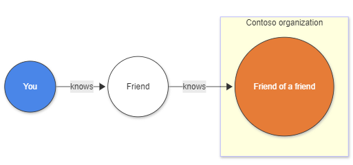
Traditional approach challenges
Without graph semantics, finding “friends-of-friends” requires multiple complex joins:
let Users = datatable (UserId: string, name: string, org: string)[]; // nodes
let Knows = datatable (FirstUser: string, SecondUser: string)[]; // edges
Users
| where org == "Contoso"
| join kind=inner (Knows) on $left.UserId == $right.FirstUser
| join kind=innerunique(Users) on $left.SecondUser == $right.UserId
| join kind=inner (Knows) on $left.SecondUser == $right.FirstUser
| join kind=innerunique(Users) on $left.SecondUser1 == $right.UserId
| where UserId != UserId1
| project name, name1, name2
Graph semantics solution
KQL graph semantics simplifies this significantly. The make-graph operator creates a directed graph, while the graph-match operator expresses the pattern concisely:
let Users = datatable (UserId:string , name:string , org:string)[]; // nodes
let Knows = datatable (FirstUser:string , SecondUser:string)[]; // edges
Knows
| make-graph FirstUser --> SecondUser with Users on UserId
| graph-match (user)-->(middle_man)-->(friendOfAFriend)
    where user.org == "Contoso" and user.UserId != friendOfAFriend.UserId
    project contoso_person = user.name, middle_man = middle_man.name, kusto_friend_of_friend = friendOfAFriend.name
Log data insights
Log data analysis often requires extracting insights from flat tables containing time-series information. Converting this data to a graph structure requires identifying relevant entities and relationships. Consider a table called rawLogs containing web server request information:
let rawLogs = datatable (rawLog: string) [
    "31.56.96.51 - - [2019-01-22 03:54:16 +0330] \"GET /product/27 HTTP/1.1\" 200 5379 \"https://www.contoso.com/m/filter/b113\" \"some client\" \"-\"",
    "31.56.96.51 - - [2019-01-22 03:55:17 +0330] \"GET /product/42 HTTP/1.1\" 200 5667 \"https://www.contoso.com/m/filter/b113\" \"some client\" \"-\"",
    "54.36.149.41 - - [2019-01-22 03:56:14 +0330] \"GET /product/27 HTTP/1.1\" 200 30577 \"-\" \"some client\" \"-\""
];
Creating a graph from log data
Model the graph by treating source IP addresses as nodes and web requests to resources as edges. Use the parse operator to extract required columns:
let parsedLogs = rawLogs
    | parse rawLog with ipAddress: string " - - [" timestamp: datetime "] \"" httpVerb: string " " resource: string " " *
    | project-away rawLog;
let edges = parsedLogs;
let nodes =
    union
        (parsedLogs
        | distinct ipAddress
        | project nodeId = ipAddress, label = "IP address"),
        (parsedLogs | distinct resource | project nodeId = resource, label = "resource");
let graph = edges
    | make-graph ipAddress --> resource with nodes on nodeId;
This creates a directed graph where nodes are IP addresses or resources, and edges represent requests with timestamp and HTTP verb properties:
Query patterns for recommendations
Use graph-match to create simple recommendations based on resources requested by other IP addresses:
graph
| graph-match (startIp)-[request]->(resource)<--(otherIP)-[otherRequest]->(otherResource)
    where startIp.label == "IP address" and //start with an IP address
    resource.nodeId != otherResource.nodeId and //recommending a different resource
    startIp.nodeId != otherIP.nodeId and //only other IP addresses are interesting
    (request.timestamp - otherRequest.timestamp < 5m) //filter on recommendations based on the last 5 minutes
    project Recommendation=otherResource.nodeId
Output:
| Recommendation |
|---|
| /product/42 |
This demonstrates how graph semantics can extract meaningful insights from raw log data.
Resource graph exploration
Resource graphs enable efficient exploration and querying of resources at scale, supporting governance, management, and security requirements. These graphs continuously update as resources change, providing dynamic tracking of your resource inventory.
Enterprise resource management challenges
Consider an enterprise with complex cloud infrastructure containing:
- Virtual machines, databases, storage accounts, and networking components
- User identities with varying permissions across multiple environments
- Complex resource hierarchies spanning different organizational units
The key challenge lies in efficiently managing and querying this extensive resource inventory for security compliance and access control.
Graph-based solutions
KQL graph semantics enables security administrators to model complex resource hierarchies and permission structures as graphs. This approach supports powerful queries that can:
- Trace access paths from users through groups to resources
- Identify overprivileged accounts and potential security vulnerabilities
- Detect configuration issues in resource permissions
- Validate compliance with organizational policies
For enterprise-scale resource graphs, materialized views can represent the current state of nodes and edges, enabling both real-time analysis and historical queries of how resources and permissions have evolved over time.
For detailed examples and sample code, see the Resource Graph samples on GitHub.
Multi-domain security analysis
Security operations often require analyzing relationships across multiple domains simultaneously. The “Graph of Graph” approach enables modeling and analyzing interconnected data structures by combining separate graph domains: identity, network, and asset graphs.
Multi-domain analysis methodology
This methodology maintains separation between domain-specific graphs while enabling sophisticated cross-domain analysis through query composition. Consider a scenario where an organization needs to detect sophisticated attacks using:
- Identity graph - Modeling users, groups, and permissions to understand access rights
- Network graph - Representing devices and connections to detect unusual network patterns
- Asset graph - Cataloging resources and sensitivity levels to assess potential impact
Advanced security insights
By traversing relationships across these domains, security analysts can identify attack paths invisible when examining each domain separately. This approach excels at:
- Detecting lateral movement across network segments
- Identifying privilege escalation attempts via group membership changes
- Discovering data exfiltration from high-sensitivity resources
- Correlating authentication patterns with resource access
For detailed examples and implementation guidance, see the Graph of Graph samples on GitHub.
Time series and graph analytics

Temporal anomaly detection with context
Time-series data often contains temporal patterns indicating normal or anomalous behavior. When combined with graph structures, these patterns gain meaningful context through relationship and access path analysis.
Security applications
In security contexts, this integration identifies potentially malicious activities through:
- Authentication anomaly detection - Flagging logins deviating from usual patterns (time, location, frequency)
- Access path analysis - Determining what sensitive resources anomalous users can reach through permission chains
- Impact assessment - Evaluating the potential blast radius of unusual activity
Broader applications
Beyond security, this approach applies to:
- IoT systems - Correlating device anomalies with connected infrastructure
- Business operations - Linking transaction anomalies with organizational structures
- IT infrastructure - Connecting performance anomalies with service dependencies
For implementation examples and detailed code samples, see the Time Series and Graph samples on GitHub.
Digital twins and graph historization
Digital twins provide virtual representations of physical objects or systems, enabling precise modeling and simulation of real-world entities. Graph semantics in KQL excels in digital twin scenarios because relationships between entities—facilities, equipment, sensors, and people—naturally form graph structures.
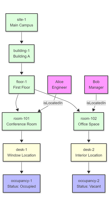
Digital twin capabilities with KQL
Graph semantics enables comprehensive digital twin modeling through:
- Hierarchical modeling - Representing complex facility and equipment hierarchies
- Multi-entity relationships - Connecting physical assets, virtual representations, and human operators
- Real-time state tracking - Monitoring occupancy, equipment status, and environmental conditions
- Cross-domain analysis - Correlating physical space utilization with operational metrics
Graph historization for temporal analysis
A critical aspect of digital twin management is capturing and analyzing temporal changes. By historizing graph changes, organizations can:
- Track evolution over time - Monitor how physical spaces and systems change
- Conduct historical analysis - Identify patterns and trends in utilization and performance
- Compare historical states - Detect anomalies or measure improvements across time periods
- Develop predictive models - Use historical utilization patterns for future planning and optimization
Implementation benefits
This approach enables organizations to:
- Monitor space utilization patterns and optimize facility management
- Track equipment performance and predict maintenance needs
- Analyze environmental conditions and their impact on operations
- Correlate human behavior patterns with physical infrastructure usage
For detailed implementation examples and code samples, see the Digital Twins samples on GitHub.
Related content
- Graph semantics overview
- Best practices for KQL graph semantics
- Graph function
- make-graph operator
- Azure Kusto Graph Samples on GitHub
- Advanced KQL graph capabilities for security analysis
- Digital twins with KQL graph semantics
- Graph semantics overview
- Best practices for KQL graph semantics
- make-graph operator
- Azure Kusto Graph Samples on GitHub
- Advanced KQL graph capabilities for security analysis
- Digital twins with KQL graph semantics